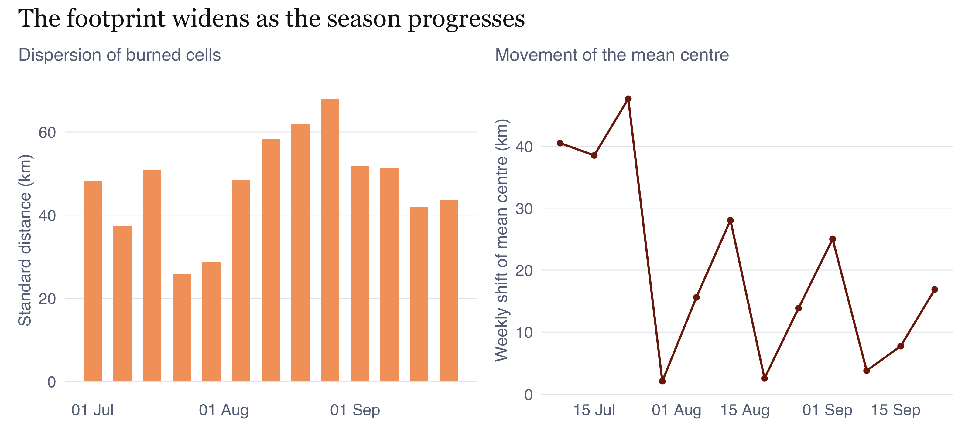
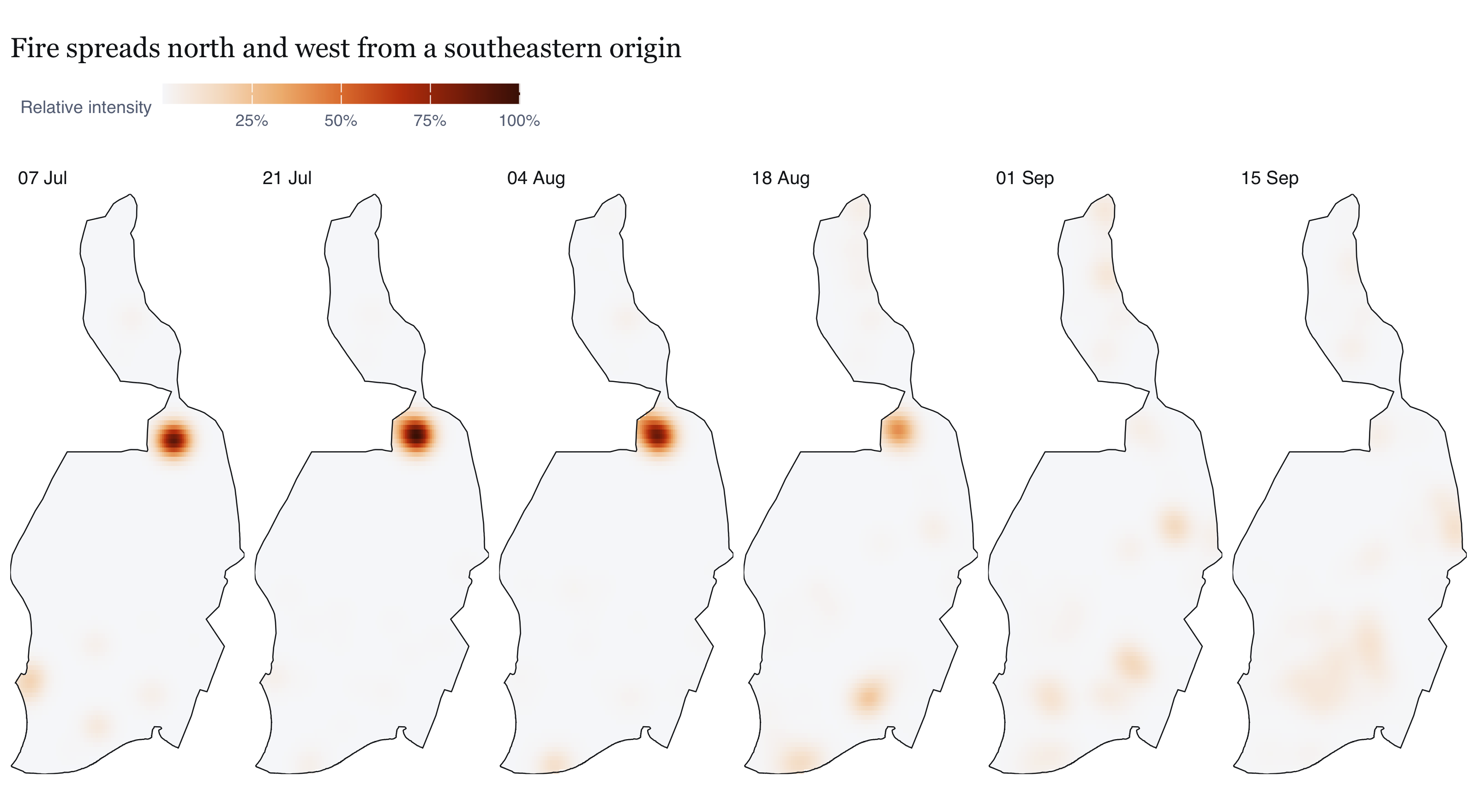
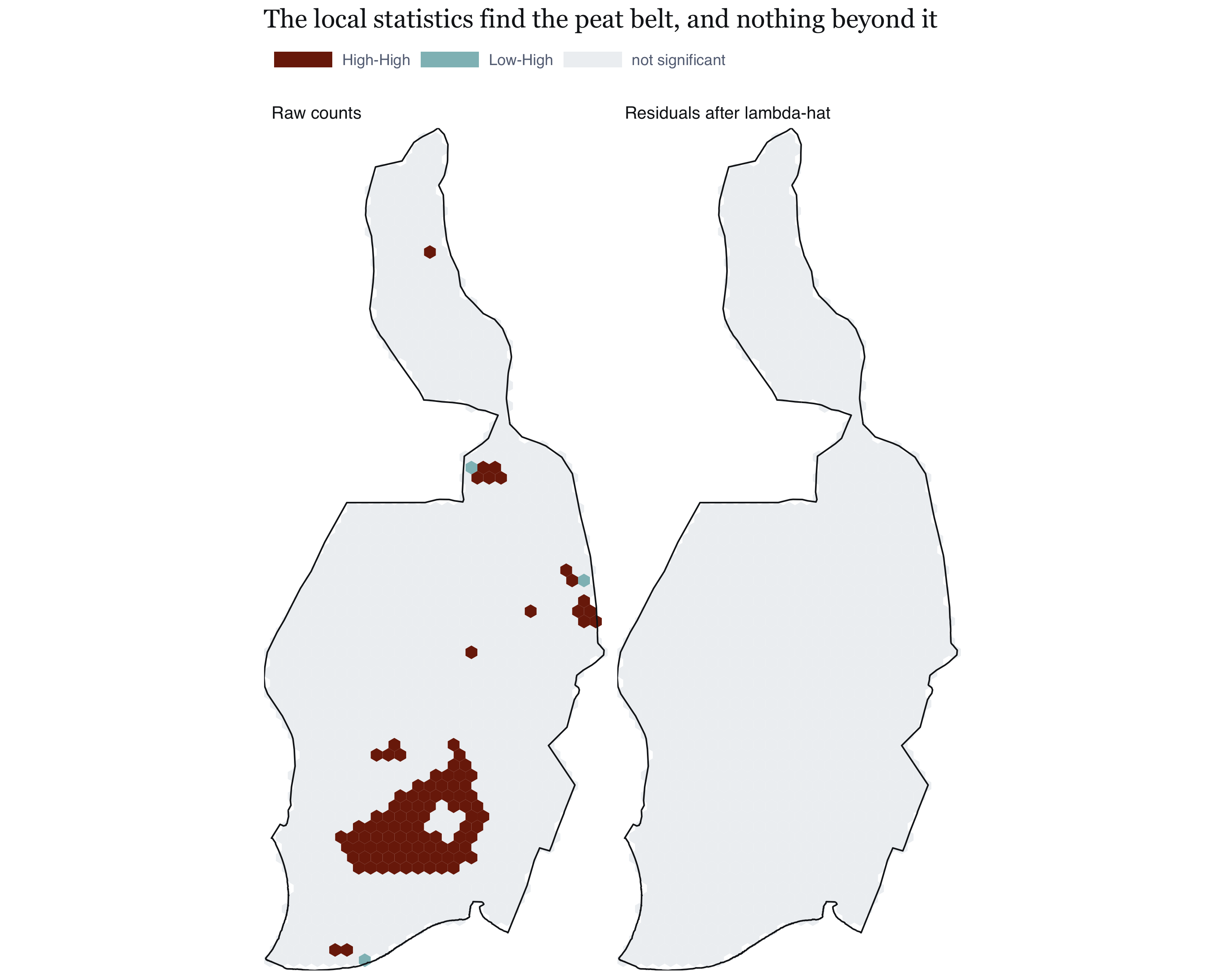
---
title: "Take-home Exercise 1: Geospatial Analytics for Public Safety"
subtitle: "First- and second-order point-pattern analysis of VIIRS active-fire detections in Pulang Pisau Regency, Central Kalimantan, 1 July to 25 September 2026"
description: |
A first- and second-order point-pattern analysis of VIIRS active-fire detections
in Pulang Pisau Regency, Central Kalimantan, 1 July to 25 September 2026.
author:
- name: Jedidiah Asaf Tallulembang
affiliation: "ISSS626 Geospatial Analytics and Applications"
date: last-modified
format:
html:
toc: true
toc-depth: 3
code-fold: true
code-summary: "code"
code-tools: true
fig-width: 8
fig-height: 5
fig-dpi: 200
fig-align: left
tbl-cap-location: bottom
fig-cap-location: bottom
number-sections: true
abstract: |
I analyse VIIRS active-fire detections over Pulang Pisau Regency, Central
Kalimantan, across the 2026 dry season, asking where they concentrate, whether
they interact beyond that concentration, and what a fire agency could honestly do
with the answer.
One distinction shaped everything. A VIIRS hotspot is a 375 m pixel seen during a
single overpass, not a fire, and I measured the consequence: the raw count
overstates distinct burning locations by a factor of about 3.4. Testing that
pattern against complete spatial randomness rejects the null overwhelmingly and
establishes nothing, because the sensor guarantees the result. I moved the unit of
analysis to the 375 m cell and the null to an inhomogeneous Poisson process, with
the reference intensity re-estimated for every simulated pattern. That test could
fail. It does not.
Clustering beyond the trend peaks at about 440 m and decays to within 10% of no
excess only by roughly 7 km. A Thomas process fitted after the trend is removed
puts the cluster standard deviation near a kilometre, with a parametric bootstrap
interval of 0.90 to 1.03 km and 2.2 to 2.5 km holding most of a cluster. Proximity
to plantation and farmland is the strongest covariate, recovering 90% of the
explanatory power of the full model from one term. An areal
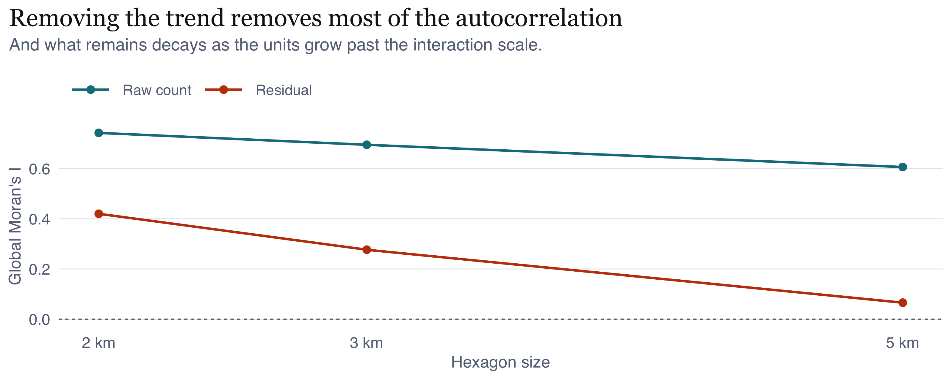
analysis agrees from different machinery: Moran's I on hexagons falls from 0.69 on
raw counts to 0.28 once the intensity is removed, and to 0.07 as the hexagons grow
past the interaction scale. A Knox permutation test finds space-time interaction
concentrated within a few hundred metres and a few days.
Three of my own conclusions were wrong and are corrected in place, because each
correction is more informative than the claim it replaced. A 5 km distance cap put
the end of dependence at 2 km when it is nearer 7. A covariate set of roads and
waterways made access look dominant until land cover showed fire tracking cleared
and cultivated ground instead. And I had recorded that the API's ninety-day
retention made it impossible to judge whether 2026 was severe, which was a wrong
inference from one year's worth of empty queries: the archive serves earlier years
normally, and pulling the identical window back to 2013 puts 2026 second of
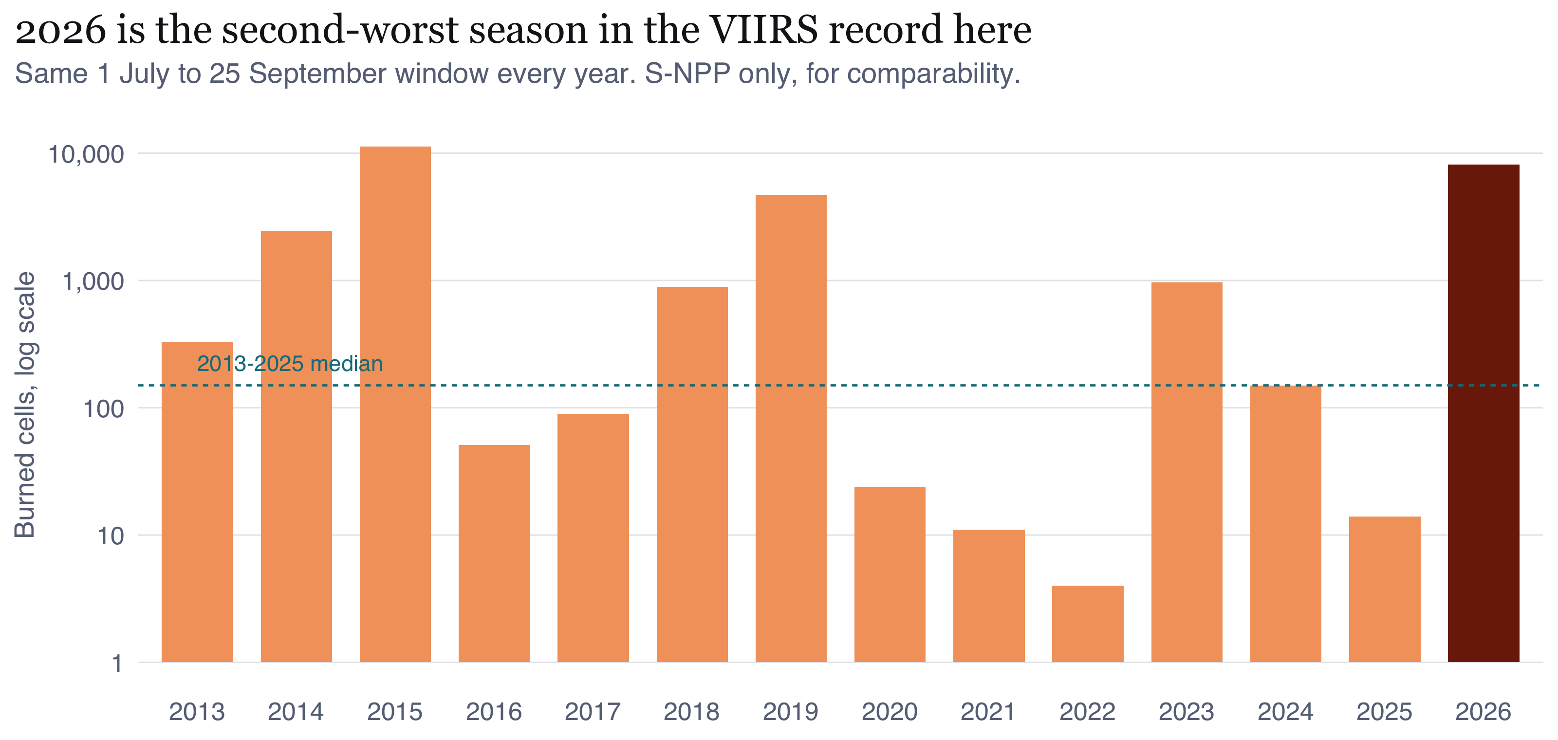
fourteen, at roughly fifty times the median. What follows describes a severe
season, not a typical one.
execute:
echo: true
---
::: {.pill-row}
[R]{.pill} [sf]{.pill} [spatstat]{.pill} [NASA FIRMS]{.pill} [KDE]{.pill} [Kinhom]{.pill} [Knox test]{.pill} [Thomas process]{.pill}
:::
[**Executive summary, 10 slides**](slides.qmd){.btn} · [**Repository**](https://github.com/jediasaf/isss626-coursework/tree/main/Take-home_Ex/Take-home_Ex01)
```{r setup}
#| include: false
knitr::opts_chunk$set(fig.showtext = FALSE, out.width = "100%")
suppressPackageStartupMessages({
library(dplyr); library(tidyr); library(sf); library(ggplot2); library(glue)
library(knitr); library(spatstat.geom); library(spatstat.explore)
library(spatstat.model); library(spatstat.random); library(patchwork)
})
source("R/00_config.R")
source("R/helpers.R")
P <- readRDS(file.path(DIR_DERIVED, "prepared.rds"))
FO <- readRDS(file.path(DIR_DERIVED, "firstorder.rds"))
SO <- readRDS(file.path(DIR_DERIVED, "secondorder.rds"))
ST <- readRDS(file.path(DIR_DERIVED, "spacetime.rds"))
CM <- readRDS(file.path(DIR_DERIVED, "covariates_models.rds"))
EX <- readRDS(file.path(DIR_DERIVED, "extended.rds"))
TH <- readRDS(file.path(DIR_DERIVED, "thomas.rds"))
MY <- readRDS(file.path(DIR_DERIVED, "multiyear.rds"))
AN <- readRDS(file.path(DIR_DERIVED, "anisotropy.rds"))
BC <- readRDS(file.path(DIR_DERIVED, "cover_boot.rds"))
RK <- readRDS(file.path(DIR_DERIVED, "residual_k.rds"))
LI <- readRDS(file.path(DIR_DERIVED, "lisa.rds"))
CS <- readRDS(file.path(DIR_DERIVED, "cover_split.rds"))
RANK <- readRDS(file.path(DIR_DERIVED, "regency_ranking.rds"))
PROBE <- readRDS(file.path(DIR_DERIVED, "retention_probe.rds"))
GAP <- readRDS(file.path(DIR_DERIVED, "gap_report.rds"))
win_sf <- P$win_sf; win_p <- P$win_p; bb <- st_bbox(win_p)
gg_win <- list(
geom_sf(data = win_p, fill = NA, colour = PAL$ink, linewidth = 0.4),
coord_sf(expand = FALSE, datum = NA),
scalebar_layer(bb), north_layer(bb), theme_map()
)
```
# Introduction and study context
Indonesian Borneo burns every dry season, and when I started reading about it I
learned that the fires which matter most for public health are not forest fires in
the ordinary sense. They are peat fires. Drained tropical peat is a metres-deep
carbon store that, once dry, smoulders below the surface for weeks. You cannot put
it out by suppressing a surface flame front, and it releases a dense particulate
smoke that carries hundreds of kilometres. So the public-safety burden is
respiratory rather than thermal: school closures, airport closures, and a
measurable excess of acute respiratory cases across Central Kalimantan and, in bad
years, across the Malacca Strait.
Pulang Pisau Regency sits at the centre of this. Its southern half was the site of
the Mega Rice Project, a 1990s programme that cut thousands of kilometres of
drainage canal into deep peat and was then abandoned. The canals are still there,
the water table is still lowered, and the land is still unusually combustible. That
is why I did not treat the regency as just a convenient study window. It is a place
where the link between land management and public-safety outcomes is about as
visible as it gets.
Fire detections are point events in space and time, so point-pattern analysis is
the obvious tool. What I wanted to work out in this exercise is what that tool can
honestly support once you take the data seriously.
## The problem the data handed me {#sec-not-a-fire}
A VIIRS active-fire detection is not a fire. It is a 375 m pixel where a radiometer
measured a thermal anomaly during one overpass. A peat fire covering ten square
kilometres fills dozens of those pixels in a single pass, and between them the two
satellites pass overhead about four times a day, so the same fire is recorded again
and again. The detection set samples the sensor's view of fire. Any statistic I
compute on it is partly a measurement of the instrument.
That ruins the textbook second-order question. Asking whether the pattern is
clustered relative to complete spatial randomness has an answer before I compute
anything: yes, overwhelmingly, and it would still be yes if fires were sited at
random, because each one produces a burst of adjacent detections. I did not want to
build a report on a rejection that was guaranteed.
Two changes follow, and they are the methodological content of this exercise. The
unit of analysis becomes the 375 m cell, not the detection. The null becomes an
inhomogeneous Poisson process, not complete spatial randomness. @sec-second-order is where
that earns its keep.
# Research questions and objectives {#sec-questions}
I set four questions, each with a null and a reason for asking it. I wrote these
before running the second-order analysis, so the report can be read as a test of
them rather than as a description of whatever came out.
**Q1. How does the intensity of fire detection vary across the regency, and at what
spatial scale is that variation stable?**
First-order. I ask it because a fire agency allocates fixed resources to places, so
what is useful to them is a surface, not a test. I added the scale qualifier because
a kernel estimate can be made to show almost any structure depending on the
bandwidth, so I do not think the question is answerable unless I also defend that
choice.
**Q2. How does intensity vary in time, and is the temporal signal a property of fire
activity or of the observing system?**
First-order. I split this out because the two satellites observe at fixed local
times, so any apparent daily cycle is a sampling artefact. I wanted to be sure I did
not read the orbit as fire behaviour.
**Q3. Once large-scale variation in intensity is accounted for, is there residual
interaction between events, and over what distance?**
Second-order. My null is an inhomogeneous Poisson process with intensity
$\hat{\lambda}(u)$ estimated by kernel smoothing. Rejecting this null tells me
something that rejecting complete spatial randomness does not, because the
inhomogeneous null already contains everything my first-order analysis found. The
"over what distance" part is the bit with operational value, and it is also the part
I initially got wrong.
**Q4. Is there space-time interaction, over and above the separate spatial and
temporal patterns?**
Second-order, spatio-temporal. My null is random labelling: I hold the observed
locations and the observed set of dates fixed and permute only the pairing between
them. This conditions on both marginal patterns, which matters, because it means a
rejection cannot be explained away by the seasonal ramp or by the spatial
concentration. I already know both of those exist.
I added a fifth question as a value-added extension in @sec-valueadded, because the four
above tell me clustering exists without telling me what it is organised around or
how big a cluster actually is.
# Data and study design
## Sources
```{r tbl-sources}
#| label: tbl-sources
#| tbl-cap: "The data I used, as accessed. Both sources are re-creatable by running `R/01_acquire.R`. I pinned the geoBoundaries release to a commit hash so the boundary geometry cannot change underneath my analysis."
tibble::tribble(
  ~Item, ~Detail,
  "Event data", "NASA FIRMS, VIIRS 375 m Collection 2, near-real-time (NRT)",
  "Platforms", "Suomi NPP and NOAA-20, both retained",
  "Access route", "FIRMS `area` REST API, CSV, 5-day request blocks",
  "Access date", format(ACCESS_DATE, "%d %B %Y"),
  "Spatial extent requested", "108.5 to 119.1 E, 5.2 S to 4.5 N (all Kalimantan)",
  "Boundaries", "geoBoundaries gbOpen Indonesia ADM1 and ADM2, commit 9469f09",
  "Boundary vintage", "2020, sourced from BPS Statistics Indonesia via OCHA",
  "Boundary licence", "CC BY 3.0 IGO",
  "Covariates", "OpenStreetMap via Overpass: `highway`, `waterway`",
  "Software", glue("R {getRversion()}, sf {packageVersion('sf')}, spatstat.explore {packageVersion('spatstat.explore')}")
) |> kable()
```
## Why I chose this regency
I chose the study window with a rule applied to the whole island, after downloading
data for all 56 Kalimantan regencies and cities and screening it for confidence.
The rule: **the highest detection density among regencies large enough to support
second-order estimation to a 5 km lag**, which I operationalised as an area above
5,000 km².
I used density rather than raw count because intensity relative to window area is
what governs how much signal a point pattern carries. I added the size floor because
a 5 km lag inside a small window starts to approach the window's own dimension, and
at that point edge effects dominate every second-order estimate I would compute.
```{r tbl-rank}
#| label: tbl-rank
#| tbl-cap: "The ten Kalimantan regencies with the most retained VIIRS detections, 1 July to 25 September 2026. Ketapang leads on count; Pulang Pisau leads on density among regencies above the 5,000 km² size floor, which is the selection rule applied. Kota Palangka Raya's very high density in a small window illustrates why the floor is needed."
RANK |> slice_head(n = 10) |>
  transmute(
    Regency = shapeName, Province = province,
    Detections = fmt_n(n_detections),
    `Area (km²)` = fmt_n(round(area_km2)),
    `Per 1,000 km²` = fmt_n(round(per_1000km2))
  ) |> kable(align = "llrrr")
```
Pulang Pisau wins on that rule outright, at
`r round(RANK$per_1000km2[RANK$shapeName == STUDY_REGENCY])` detections per
1,000 km². Two alternatives were seriously considered and rejected, and the
reasons are recorded because a choice is only reviewable alongside them.
**Ketapang** beat it on absolute count, with
`r fmt_n(RANK$n_detections[RANK$shapeName == "Ketapang"])` detections against Pulang
Pisau's `r fmt_n(RANK$n_detections[RANK$shapeName == STUDY_REGENCY])`. I did not
choose it because it covers
`r fmt_n(round(RANK$area_km2[RANK$shapeName == "Ketapang"]))` km², slightly over
three times the area, and ranks second on density. Its bigger count is mostly just
a bigger window.
**Kota Palangka Raya** has the highest density of any unit at
`r fmt_n(round(RANK$per_1000km2[RANK$shapeName == "Kota Palangka Raya"]))` per
1,000 km², but covers only
`r fmt_n(round(RANK$area_km2[RANK$shapeName == "Kota Palangka Raya"]))` km². A 5 km
lag there is a large fraction of the window's own width, so edge effects would drive
my second-order results rather than the fires.
Pulang Pisau also comes rank
`r which(RANK$shapeName == STUDY_REGENCY)` of `r nrow(RANK)` on raw count, so I am
not selecting some obscure unit to make the rule work. Its window of
`r fmt_n(round(P$area_km2))` km², at
`r round((bb["xmax"]-bb["xmin"])/1000)` km by
`r round((bb["ymax"]-bb["ymin"])/1000)` km, comfortably supports estimation to a
5 km lag.
My first pass picked the regency from a seven-day sample, where Pulang Pisau led on
count. Over the full 87 days it does not. Ketapang does. I restated the rule against
the complete record and applied it again. A rule chosen after you have seen which
unit it favours is not a rule, so the sequence is recorded here for the reader to
judge.
## Point event definition
I define an event as **one 375 m grid cell in which at least one qualifying VIIRS
detection was recorded**. Qualifying means all of the following, and I have given
the reason for each rather than just the rule.
```{=html}
<dl class="assump">
<dt>Sensor and product</dt>
<dd>VIIRS 375 m I-band, Collection 2, S-NPP or NOAA-20. MODIS is excluded: its
1 km footprint is coarser than the distances this analysis is about, so including
it would blur the very scale under study.</dd>
<dt>Confidence</dt>
<dd>Nominal or high. Low-confidence detections are dropped. They are dominated by
small or cool anomalies and by edge-of-scan geometry, so retaining them would
make apparent intensity vary with viewing angle rather than with fire.</dd>
<dt>Coordinates</dt>
<dd>Present, finite, within valid latitude and longitude ranges, and not the
(0, 0) sentinel that some pipelines emit for a failed geolocation.</dd>
<dt>Timestamp</dt>
<dd>A parseable UTC acquisition time. Converted to WITA (UTC+8), because the
definition of a fire day and any reading of diurnal behaviour must be local.</dd>
<dt>Location</dt>
<dd>Strictly within the Pulang Pisau polygon. This also serves as the offshore
screen, since the polygon is terrestrial.</dd>
<dt>Not a fixed installation</dt>
<dd>See the persistence screen below. This substitutes for a field the NRT
product does not carry.</dd>
<dt>Deduplicated</dt>
<dd>Exact duplicate records removed, then collapsed to one event per 375 m cell
per local day.</dd>
</dl>
```
I build three patterns from the same screened detections, because which unit is
right depends on which question I am asking:
| Pattern | Unit | Used for |
|---|---|---|
| `ppp_all` | every retained detection | sensitivity checks only |
| `ppp_daycell` | one event per 375 m cell per local day | spatio-temporal analysis |
| `ppp_cell` | one event per 375 m cell over the window | primary spatial analysis |
I use `ppp_cell` as the primary spatial pattern because it removes the
repeat-detection inflation I described in @sec-not-a-fire. A cell that burned for three
weeks and was detected eighty times contributes one point, not eighty.
For the representative point of each cell I take the earliest detection in it. That
is deterministic and it keeps a real sensor coordinate. I considered snapping to
cell centres and rejected it, because that would impose a regular lattice and
manufacture apparent regularity at small lags, which would contaminate exactly the
statistic the rest of the report depends on.
## Spatial study window
My window is the Pulang Pisau administrative polygon, unbuffered, in WGS 84 /
UTM zone 49S (EPSG:32749).
Projecting is not optional here. Every second-order statistic I use is a function of
Euclidean distance in metres, and at this latitude one degree of longitude is about
111 km while one degree of latitude is about 110.6 km. If I worked in degrees I
would be building a systematic anisotropy into every distance I compute. Zone 49S is
the right one for a regency centroid at 113.96°E, which sits inside the zone's 108°E
to 114°E span. I checked the eastern edge, which reaches 114.35°E and is marginally
outside, and the resulting scale error is below 0.1%, so it does not matter at the
kilometre scales I work at.
I used the administrative boundary rather than a buffered or natural window because
the management question is administrative: a regency fire agency has jurisdiction to
that line. The cost is a real edge effect, since fires obviously do not stop at a
boundary, and I handle it with edge correction rather than pretending it is not
there (@sec-assumptions).
## Temporal study window
**1 July to 25 September 2026, 87 days.** The lower bound was imposed on me rather
than chosen, and I want to state the constraint precisely, because it is the kind of
thing that is easy to misrepresent by accident.
```{r tbl-probe}
#| label: tbl-probe
#| tbl-cap: "Retention probe. Single-day FIRMS NRT queries over a Kalimantan-wide box. Exactly zero detections across a 10.6° by 9.7° box for every sampled date from January to 30 June is not a physically credible result for Borneo, so the zeros are read as absence of coverage. The standard-processing archive, queried for the same region in August, also returns zero rows: it has not yet been built for 2026."
PROBE$nrt |> transmute(Date = format(date, "%d %b %Y"),
                       `Detections returned` = fmt_n(n)) |> kable(align = "lr")
```
The FIRMS `area` REST endpoint serves near-real-time granules on a rolling retention
of roughly 90 days, and the standard-processing product has not been produced for
2026 yet, because NRT granules are only replaced by standard science quality data
after a lag of about five months. So the earliest day the API will give me is 1 July
2026, which I located to the day with the probe above rather than assuming it. The
upper bound is my choice: the last complete UTC day before I accessed the data, so
that no partially observed day enters the daily series and shows up as a fake
decline.
I should be precise about what that constraint is and is not, because it would be
easy to overstate it. **The 90-day limit belongs to the API, not to the data.** FIRMS
also publishes an archive download service covering VIIRS S-NPP from 20 January 2012
and NOAA-20 from 1 April 2018. It is a request form rather than a REST endpoint: it
authenticates through an Earthdata login or an emailed verification code, and it
delivers the extract by email afterwards. That is a perfectly obtainable dataset, and
the reason this report does not use it is a scripting constraint rather than a data
constraint. My pipeline is built to run unattended from a single key, and the archive
service cannot be driven that way.
The honest statement is therefore that I chose a 87-day window served by the API over
a multi-year window that would have required an out-of-band request. @sec-limitations records what that cost me.
I want to be careful not to oversell the window. It is what was available. But it
does happen to span the onset, escalation and peak of the 2026 dry season, which is
the period a fire agency actually acts over. If the retention limit had cut off the
peak instead of the wet-season baseline I would have had to change the study design
entirely. The honest cost is that I cannot make any wet-season comparison, so nothing
in this report speaks to the seasonal amplitude of fire activity, only to its
structure within one season. I repeat that in @sec-limitations because it is a real limit
on what I can claim.
## My completeness audit, and a real outage
Counting downloaded rows does not establish completeness. The failure I was worried
about is a request that returns empty, which looks exactly like a day on which
nothing burned and would appear in the analysis as a drop in fire activity that
never happened.
The audit is built around one expectation: across an 87-day dry season, each
platform should record at least one detection somewhere in Kalimantan every day. An
island-sized box is never entirely without fire. Any day where a platform
contributes nothing is a candidate failure.
```{r tbl-gap}
#| label: tbl-gap
#| tbl-cap: "Completeness audit. Local dates on which one VIIRS platform contributed no detection anywhere in the Kalimantan bounding box. Each was re-queried four times with backoff by `R/01b_fill_gaps.R`, and each returned empty again, so these are not failed requests."
GAP$missing_after |> transmute(Date = format(dt, "%d %B %Y"),
                               `Platform absent` = platform) |> kable(align = "ll")
```
```{r}
#| label: gap-inline
#| include: false
bad <- GAP$missing_after$dt
ev_bad <- sum(P$daily_daycell$n_events[P$daily_daycell$date_local %in% bad])
ev_all <- sum(P$daily_daycell$n_events)
```
Six of the seven dates are consecutive, which pointed at an outage rather than a
flaky connection. Re-querying confirmed it. Suomi NPP returns empty for 11 to 16
July and for 3 August however many times I ask, so the absence is in the FIRMS
record itself. On those seven days the analysis rests on NOAA-20 alone and counts
are depressed by roughly one platform's contribution.
The consequence is small, but I do not want to write it off as nothing. Those dates
carry
`r fmt_n(ev_bad)` of `r fmt_n(ev_all)` events, or
`r sprintf("%.2f%%", 100 * ev_bad / ev_all)` of the record, and all of them fall in
the near-zero early season before the dry-season ramp. Mean daily events on the
affected dates are `r round(mean(P$daily_daycell$n_events[P$daily_daycell$date_local %in% bad]), 1)`
against `r round(mean(P$daily_daycell$n_events[P$daily_daycell$date_local >= as.Date("2026-07-01") & P$daily_daycell$date_local <= as.Date("2026-07-26") & !(P$daily_daycell$date_local %in% bad)]), 1)`
on nearby unaffected July dates, which is consistent with losing one platform on
very small counts. No conclusion I draw turns on those seven days, but the reader
should treat the early-season part of my daily series as a slight underestimate.
# Data preparation and quality assessment
## The audit trail
I counted every exclusion. The table below is generated by the pipeline rather than
typed in by me, so it cannot drift away from what the code actually did.
```{r tbl-qa}
#| label: tbl-qa
#| tbl-cap: "My screening audit. Each row is one rule applied in `R/02_prepare.R`, in the order I applied it. Counts are rows of the detection table, before I collapse to cell-level events."
P$qa |> transmute(Step = step, Rule = rule,
                  `In` = fmt_n(n_in), Removed = fmt_n(n_removed), `Out` = fmt_n(n_out)) |>
  kable(align = "llrrr")
```
Three things I want to point out about this table.
The biggest single reduction is the spatial clip, and that is expected. I downloaded
all of Kalimantan so that I could justify my choice of regency against the
alternatives, and the overwhelming majority of those detections are outside Pulang
Pisau.
The coordinate and timestamp screens removed nothing at all. I am flagging that
rather than skipping past it, because in my experience a cleaning step that catches
nothing is often a cleaning step that is not actually testing what it says it is. I
checked mine against deliberately broken records while developing the pipeline, and
they do fire. The FIRMS product is simply well-formed here: every record had finite
coordinates in range and a parseable timestamp. I kept the screens in because I want
the pipeline to be re-runnable against other windows and products where that will
not be true.
The confidence screen removed
`r percent(P$qa$n_removed[P$qa$step == "03 confidence"] / P$qa$n_in[P$qa$step == "03 confidence"], accuracy = 0.1)`
of records, and exact duplicate removal a further
`r fmt_n(P$qa$n_removed[P$qa$step == "06 exact duplicates"])` rows, confirming
that the API does deliver a small number of repeated granule records.
```{r tbl-conf}
#| label: tbl-conf
#| tbl-cap: "Confidence classes among detections surviving the coordinate and timestamp screens, before the confidence screen itself is applied. VIIRS confidence is categorical, not a percentage."
P$conf_tab |> transmute(Confidence = confidence, Detections = fmt_n(n),
                        Share = percent(n / sum(n), accuracy = 0.1)) |>
  kable(align = "lrr")
```
## The missing `type` field, and what I replaced it with
This took the longest to solve. The FIRMS standard-processing product carries a
`type` field separating vegetation fire (0) from active volcano (1), other static
land source (2) and offshore (3). The NRT product does not, which I checked against
the API response header: `r glue("column present = {P$has_type}")`. The screen it
would have given me had to be rebuilt from other evidence.
I worked through the three cases separately:
- **Volcanoes (type 1)** are not a risk at all. Borneo has no Holocene volcano, so
this screen is unnecessary not approximated. I did not need to do anything.
- **Offshore (type 3)** is already handled by my clip to the terrestrial polygon.
- **Other static land sources (type 2)** are a genuine problem. Kalimantan has
palm-oil mills, coal operations and gas flares, and all of them show up as
persistent thermal anomalies. This is the case I actually had to solve.
My substitute is a **persistence screen**. The logic is that a vegetation fire burns
out or moves, whereas a flare stack does not. So I score each 375 m cell by the
number of distinct local dates on which it was detected, as a fraction of the 87-day
window, and drop cells above a threshold as fixed installations.
```{r tbl-persist}
#| label: tbl-persist
#| tbl-cap: "Sensitivity of the persistence screen. The adopted threshold is 60% of days, at which the screen removes nothing. The grid extends well below that value to show where the screen would begin to act, which is the evidence that it is functional rather than merely quiet."
P$persist_sens |> transmute(
  `Threshold (share of days)` = percent(threshold, accuracy = 1),
  `Cells removed` = fmt_n(n_cells),
  `Detections removed` = fmt_n(n_detections)) |> kable(align = "lrr")
```
**My screen removed nothing.** My first reaction was that I had written it wrong, so
I checked it two ways, and I now think the empty result is correct.
First, no cell comes anywhere near the threshold. The most persistent cell in the
whole window was detected on `r P$persist_max_days` of `r P$n_days` days, which is
`r percent(P$persist_max_days / P$n_days, accuracy = 0.1)`. A flare stack or mill
would be detected on most clear-sky overpasses across the entire window, so nothing
here behaves like one.
Second, I used radiative power as an independent check, because it separates the two
cases without relying on persistence at all. A fixed industrial source emits a high
and steady radiative power, while smouldering peat emits a low one.
```{r tbl-persist-top}
#| label: tbl-persist-top
#| tbl-cap: "The ten most persistently detected cells, with their mean fire radiative power. If these were industrial sources their mean FRP would sit far above the window median; instead they sit at or near it, which is the signature of recurrent low-intensity peat combustion."
P$persist_top |> transmute(
  Cell = cell, Detections = n_det, `Days detected` = n_days,
  `Share of window` = percent(day_frac, accuracy = 0.1),
  `Mean FRP (MW)` = mean_frp) |> kable(align = "lrrrr")
```
The median FRP across all my retained detections is `r round(P$frp_median_all, 1)`
MW, and the most persistent cells range from `r min(P$persist_top$mean_frp)` to
`r max(P$persist_top$mean_frp)` MW. They are not brighter than the population at
all. They are ordinary peat fires that happened to recur in the same cell.
That fits the regency's land use. Pulang Pisau is peatland and smallholder
agriculture, without the gas processing or open-cut coal operations that generate
persistent thermal anomalies elsewhere in Kalimantan. If I had picked a window in
East Kalimantan instead, I think this screen would have been doing real work.
I report the sensitivity across thresholds rather than a single number on purpose. If
the result swung sharply depending on where I put the line, that would be a decision
dressed up as a method, and the reader deserves to see which one it is.
## My evidence that a detection is not a fire
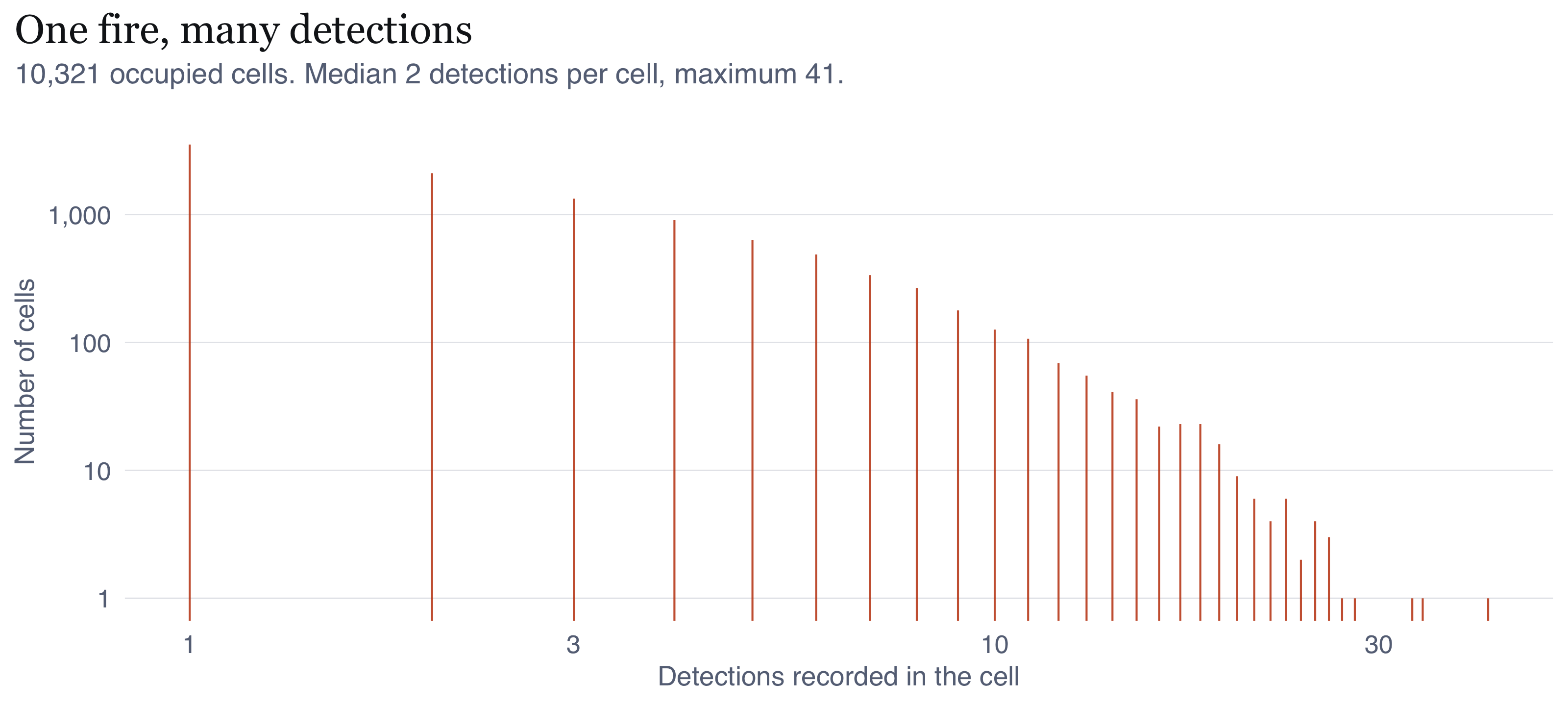
The claim I made in @sec-not-a-fire is checkable, so I checked it. If detections were
independent events, most occupied cells would be detected exactly once. They are
not.
```{r fig-mult}
#| label: fig-mult
#| fig-cap: "Detections per occupied 375 m cell over the 87-day window, log scale on both axes. If each detection were an independent event, the distribution would be concentrated at one. Instead a long tail of cells is detected tens or hundreds of times, which is the repeat-observation signature of persistent fire in a fixed pixel grid observed roughly four times daily."
#| fig-height: 3.6
mt <- P$multiplicity
ggplot(mt, aes(n_det, n_cells)) +
  geom_segment(aes(xend = n_det, yend = 0), colour = PAL$accent, linewidth = 0.35, alpha = 0.85) +
  scale_x_log10(labels = label_number(accuracy = 1)) +
  scale_y_log10(labels = label_number(big.mark = ",", accuracy = 1)) +
  labs(x = "Detections recorded in the cell", y = "Number of cells",
       title = "One fire, many detections",
       subtitle = glue("{fmt_n(sum(mt$n_cells))} occupied cells. Median {median(rep(mt$n_det, mt$n_cells))} detections per cell, ",
                       "maximum {max(mt$n_det)}.")) +
  theme_ex01()
```
```{r}
#| label: mult-stats
#| include: false
mt_v <- rep(mt$n_det, mt$n_cells)
share_once <- mean(mt_v == 1)
infl <- P$ppp_all$n / P$ppp_cell$n
```
Only `r percent(share_once, accuracy = 0.1)` of occupied cells were detected exactly
once. The mean is `r round(mean(mt_v), 1)` detections per occupied cell, so the raw
count overstates the number of distinct burning locations by a factor of about
`r round(infl, 1)`. That is the number that convinced me. Analysing the raw
detections as a point pattern would mean analysing the satellite's revisit schedule
about as much as the fire regime, which is why I made `ppp_cell` the primary unit.
```{r tbl-patterns}
#| label: tbl-patterns
#| tbl-cap: "The three patterns I built and their mean intensities. The gap between the first and third rows is the repeat-detection inflation I quantified above."
tibble::tibble(
  Pattern = c("`ppp_all`", "`ppp_daycell`", "`ppp_cell`"),
  Unit = c("retained detection", "cell-day", "cell"),
  n = c(P$ppp_all$n, P$ppp_daycell$n, P$ppp_cell$n),
  `Mean intensity (per 1,000 km²)` = round(c(P$ppp_all$n, P$ppp_daycell$n, P$ppp_cell$n) / P$area_km2 * 1000)
) |> mutate(n = fmt_n(n)) |> kable(align = "llrr")
```
## Geometry validation
I checked the boundary polygon for validity before using it. It is a single valid
polygon, so I did not need any multipart or self-intersection handling, though I ran
`st_make_valid` anyway as a defensive step. For point-in-polygon assignment I used
`st_within` rather than `st_intersects`, so a detection sitting exactly on the
boundary arc is excluded rather than double-counted against a neighbouring regency.
`spatstat`'s window conversion reported no points rejected as outside the window,
which tells me my clip and the `owin` agree.
Two things here commonly go wrong and I handled them deliberately. First, I assigned
regencies to parent provinces by testing containment of an interior representative
point in a projected coordinate system, not by nearest-feature matching. Nearest
feature would silently mis-assign any regency whose representative point fell
marginally outside its own province, and I would never have noticed. Second, I read
the 159 MB national ADM2 file through a bounding-box filter at the GDAL level rather
than loading it and subsetting afterwards, so the full national geometry is never
held in memory.
# Analytical assumptions and methodological decisions {#sec-assumptions}
Listing assumptions is easy. What I found harder, and more useful, was working out
where each one might actually fail, so I have written each with the reason I think
it could break rather than just the statement.
```{=html}
<dl class="assump">
<dt>A1. Detections are a censored observation of fire, not a sample of fires</dt>
<dd>VIIRS detects fires above a size and temperature threshold that varies with scan
angle, cloud and canopy. Smouldering sub-surface peat combustion, the dominant mode
in this landscape, is systematically under-detected because its surface signature is
weak. So what I am analysing is the pattern of <em>detectable</em> fire. That biases
against exactly the fire type I care most about for public health, and I have no
correction available within this data source. My intensity estimates are therefore a
lower bound, and their spatial variation is partly variation in detectability rather
than in fire.</dd>
<dt>A2. Cloud cover is not spatially confounded with fire location</dt>
<dd>I assume this and I cannot fully defend it. Dry-season convection over Borneo is
not spatially uniform, and smoke itself attenuates the signal. If cloud were
systematically thicker over one part of the regency, apparent intensity there would
be depressed and I would read it as less fire. I cannot establish the direction of
that bias from the detection data alone.</dd>
<dt>A3. The window is fixed and known, and events outside it are irrelevant</dt>
<dd>This is false as physics and I adopt it as a management framing. Fires cross the
regency boundary constantly. That is why I edge-correct every second-order estimate,
and why I report how sensitive my conclusions are to the correction rather than
assuming it away.</dd>
<dt>A4. The 375 m cell is the finest meaningful spatial resolution</dt>
<dd>This follows from the sensor rather than from any choice of mine. It imposes a
hard minimum separation between distinct events, and I can see it in the pair
correlation function as apparent inhibition below roughly 400 m. That inhibition is
a property of the instrument. Reading it as fires avoiding one another would be a
serious mistake, and an easy one to make.</dd>
<dt>A5. For the spatial analysis, time is collapsed</dt>
<dd>My `ppp_cell` pattern treats a cell burning in July and a cell burning in
September as the same kind of point. That is fine for "where does fire occur over a
season" and wrong for "where is fire now". I relax it in the spatio-temporal analysis.</dd>
<dt>A6. The intensity used as the inhomogeneous null is estimable from the data</dt>
<dd>This is the weakest link in my second-order analysis and I want to be upfront
about it. Estimating $\hat{\lambda}(u)$ from the same pattern I am testing lets the
estimate absorb some of the clustering under test, which pushes the envelope outward
and makes my test conservative. I mitigate it two ways: I pick a bandwidth that
describes broad trend rather than local structure, and I re-estimate
$\hat{\lambda}$ for every simulated pattern so the data and the simulations get
identical treatment. The bias that remains pushes me toward <em>failing</em> to
detect clustering, which is why I am reasonably confident the clustering I do detect
is not an artefact of this choice.</dd>
<dt>A7. Isotropy</dt>
<dd>$K$, $L$ and $g$ all assume it. I expected it to fail, on the reasoning that
peat fires spread with the wind and along canal lines. <strong>I tested it and
every part of that was wrong.</strong> There is strong directional structure below
750 m, but it is four-fold and aligned to the cardinal axes: the signature of the
375 m cell grid and of the VIIRS scan grid, not of fire. Beyond 750 m it vanishes,
leaving only a weak single-axis tilt that reaches R = 0.024 on a scale running to 1
and matches neither the drainage nor the roads. Because the four-fold component is
symmetric about the cardinal axes it cancels in direction-averaged statistics, so
it does not bias $K$, $L$ or $g$. It would wreck a directional analysis.</dd>
<dt>A8. Random labelling is the right null for space-time interaction</dt>
<dd>Permuting time labels across fixed locations conditions on both marginals. That
makes it the correct null for "is there interaction beyond the two separate
patterns" and the wrong null for "is the seasonal ramp real", which it simply
assumes. I intend that. I establish the ramp in the first-order analysis and I am not trying to
test it here.</dd>
</dl>
```
## My decisions, and what I rejected
```{r tbl-decisions}
#| label: tbl-decisions
#| tbl-cap: "The methodological decisions I made. The right-hand column records the alternative I considered and did not take, which I think is the part that makes a decision reviewable."
tibble::tribble(
  ~Decision, ~Choice, ~`Rejected alternative and why`,
  "Coordinate system", "EPSG:32749, UTM 49S", "Geographic coordinates: distance-based statistics require equal units",
  "Event unit", "one 375 m cell", "raw detections: inflates n by ~4x and measures revisit schedule",
  "Representative point", "earliest detection in cell", "cell centre: imposes a lattice, manufactures small-scale regularity",
  "Sensor", "VIIRS 375 m only", "adding MODIS 1 km: coarser than the scales under study",
  "Bandwidth", "fixed 4 km, justified against the interaction range", "bw.ppl and bw.diggle at ~0.6 km: absorb the clustering the second-order test is meant to detect",
  "Kernel", "Gaussian, isotropic", "quartic: negligible difference, less standard diagnostics",
  "Edge correction, KDE", "Diggle's correction", "none: 86 km-wide window, boundary understated",
  "Edge correction, K and L", "border", "Ripley isotropic: cost not justified at this n",
  "r range, K and L", "0 to 5 km", "larger: elongated window makes long lags unreliable",
  "Null model, primary", "inhomogeneous Poisson", "CSR: rejected trivially, uninformative",
  "Envelope construction", "lambda re-estimated per simulation", "fixed lambda: absorbs the clustering under test",
  "Significance", "MAD and DCLF global tests", "pointwise envelopes alone: inflate type-I error",
  "Simulations", glue("{SO$nsim} for envelopes, {ST$nperm} for Knox"), "fewer: coarse Monte Carlo p-value floor"
) |> kable()
```
Two of these are worth explaining properly.
**Border versus Ripley correction.** Ripley's isotropic correction is more efficient
and much more expensive, and the envelope procedure needs `r SO$nsim` re-computations
of it. At `r fmt_n(SO$n_cell)` points the efficiency lost to the border correction is
immaterial: the number of pairs contributing at each lag is already very large. A
compute trade-off, made deliberately.
**Global versus pointwise tests.** This one took me a while to get straight. A
pointwise envelope gets read at every one of several hundred values of $r$, so the
probability of at least one excursion under the null is far above the nominal level.
I still plot the pointwise envelopes, because they show me *where* on the $r$ axis
the departure sits and a single p-value cannot. But every claim of significance I
make in this report is backed by the MAD or DCLF global test, not by the band.
# First-order analysis: where, and when {#sec-first-order}
## The pattern in its region
```{r fig-context}
#| label: fig-context
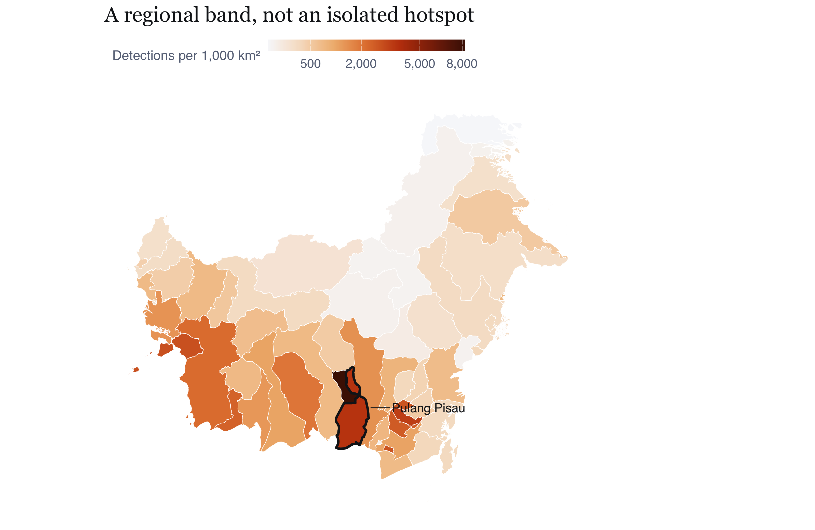
#| fig-cap: "Detection density across the 56 regencies and cities of Indonesian Borneo, 1 July to 25 September 2026, with Pulang Pisau outlined. The concentration in the southern peat belt of Central Kalimantan is the regional structure within which the study window sits. What I take from it: the choice of study window is not an outlier hunt. Pulang Pisau is the most intense cell of a coherent regional band running along the southern coastal peat domes, so findings about its internal structure plausibly transfer to its neighbours. The map also shows what the regency boundary does analytically: it cuts a continuous field of fire activity, which is why the edge corrections of Section 5 matter rather than being a formality."
#| fig-height: 5.2
kal <- readRDS(file.path(DIR_DERIVED, "kal_adm2.rds")) |> st_transform(STUDY_CRS)
kal_m <- kal |> left_join(RANK |> select(shapeName, per_1000km2), by = "shapeName") |>
  mutate(per_1000km2 = tidyr::replace_na(per_1000km2, 0))
ggplot(kal_m) +
  geom_sf(aes(fill = per_1000km2), colour = "white", linewidth = 0.18) +
  geom_sf(data = win_p, fill = NA, colour = PAL$ink, linewidth = 0.8) +
  scale_fill_intensity(name = "Detections per 1,000 km\u00b2", v = kal_m$per_1000km2) +
  annotate("text", x = bb["xmax"] + 60000, y = (bb["ymin"] + bb["ymax"]) / 2,
           label = "Pulang Pisau", hjust = 0, size = 3.1, colour = PAL$ink,
           family = "Helvetica") +
  annotate("segment", x = bb["xmax"] + 55000, xend = bb["xmax"] + 4000,
           y = (bb["ymin"] + bb["ymax"]) / 2, yend = (bb["ymin"] + bb["ymax"]) / 2,
           colour = PAL$ink, linewidth = 0.3) +
  coord_sf(datum = NA, clip = "off") +
  labs(title = "A regional band, not an isolated hotspot") +
  theme_map() + theme(plot.margin = margin(5, 90, 5, 5))
```
## The point pattern
```{r fig-points}
#| label: fig-points
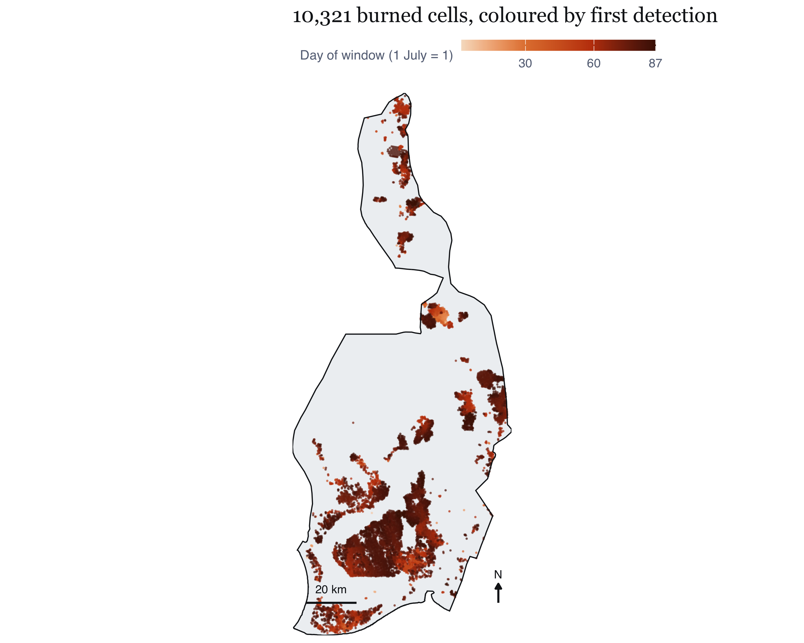
#| fig-cap: "The primary spatial pattern: one point per 375 m cell in which fire was detected. Colour shows the local date of first detection, so the map carries the season as well as the location. What I take from it: two things are immediately visible and both matter. The pattern is strongly concentrated in the southern two-thirds of the regency, which is the drained peat of the former Mega Rice Project, while the northern interior is nearly empty. Second, the colour gradient is not spatially random: earlier detections (lighter) sit disproportionately in the south and east, later ones spread north and west. That is a testable claim about space-time interaction rather than an impression, and Section 8 tests it."
#| fig-height: 6.4
pts_df <- P$fires |> st_coordinates() |> as.data.frame() |>
  bind_cols(P$fires |> st_drop_geometry() |> select(date_local))
first_seen <- P$ppp_cell
pc <- tibble(x = first_seen$x, y = first_seen$y,
             date = marks(first_seen)$date_local)
ggplot() +
  geom_sf(data = win_p, fill = PAL$ground_alt, colour = NA) +
  geom_point(data = pc, aes(x, y, colour = as.numeric(date - WINDOW_START) + 1),
             size = 0.16, alpha = 0.55) +
  scale_colour_gradientn(colours = c("#F6DFC8", "#E2803C", "#C2410C", "#4A1403"),
                         name = "Day of window (1 July = 1)",
                         breaks = c(1, 30, 60, 87)) +
  gg_win +
  labs(title = glue("{fmt_n(P$ppp_cell$n)} burned cells, coloured by first detection"))
```
## Quadrat counts, and why I do not lean on them
```{r tbl-quad}
#| label: tbl-quad
#| tbl-cap: "Chi-squared test of a homogeneous Poisson process, across quadrat resolutions. The variance-to-mean ratio (VMR) is 1 under complete spatial randomness. The verdict is identical at every resolution, which is the point: the test is not informative, it is merely arithmetically certain."
FO$quad_summary |> transmute(
  Grid = glue("{nx} x {ny}"), Quadrats = n_quadrats,
  `chi-squared` = fmt_n(round(X2)), df = df,
  VMR = vmr, `p-value` = vapply(p_value, fmt_p, character(1))) |> kable(align = "lrrrrr")
```
The chi-squared statistic exceeds its degrees of freedom by three to four orders of
magnitude at every resolution, and the variance-to-mean ratio runs from
`r min(FO$quad_summary$vmr)` to `r max(FO$quad_summary$vmr)` against a null of 1.
Complete spatial homogeneity is rejected with certainty.
It should persuade nobody. The result was guaranteed by the data-generating process in @sec-not-a-fire, and by the geography: a regency that is half drained peatland and
half intact landscape cannot have uniform fire intensity. Quadrat counts also
inherit an arbitrary origin and cell size and discard everything within a quadrat.
The one useful column is the VMR, which says *how far* from uniform the pattern is
at each scale instead of answering a question I already knew the answer to.
## Bandwidth selection, and why I rejected cross-validation
Kernel density estimation does the work here, and the bandwidth decides what it
shows. This took longer than any other single choice in the report.
```{r tbl-bw}
#| label: tbl-bw
#| tbl-cap: "Bandwidth selectors compared on the primary pattern, ordered as computed. The spread is a factor of roughly eighteen from smallest to largest, which is why reporting a single surface without this table would conceal the most consequential choice in the first-order analysis."
FO$bw_tab |> transmute(Selector = selector, `sigma (m)` = round(sigma_m),
                       `sigma (km)` = sigma_km) |> kable(align = "lrr")
```
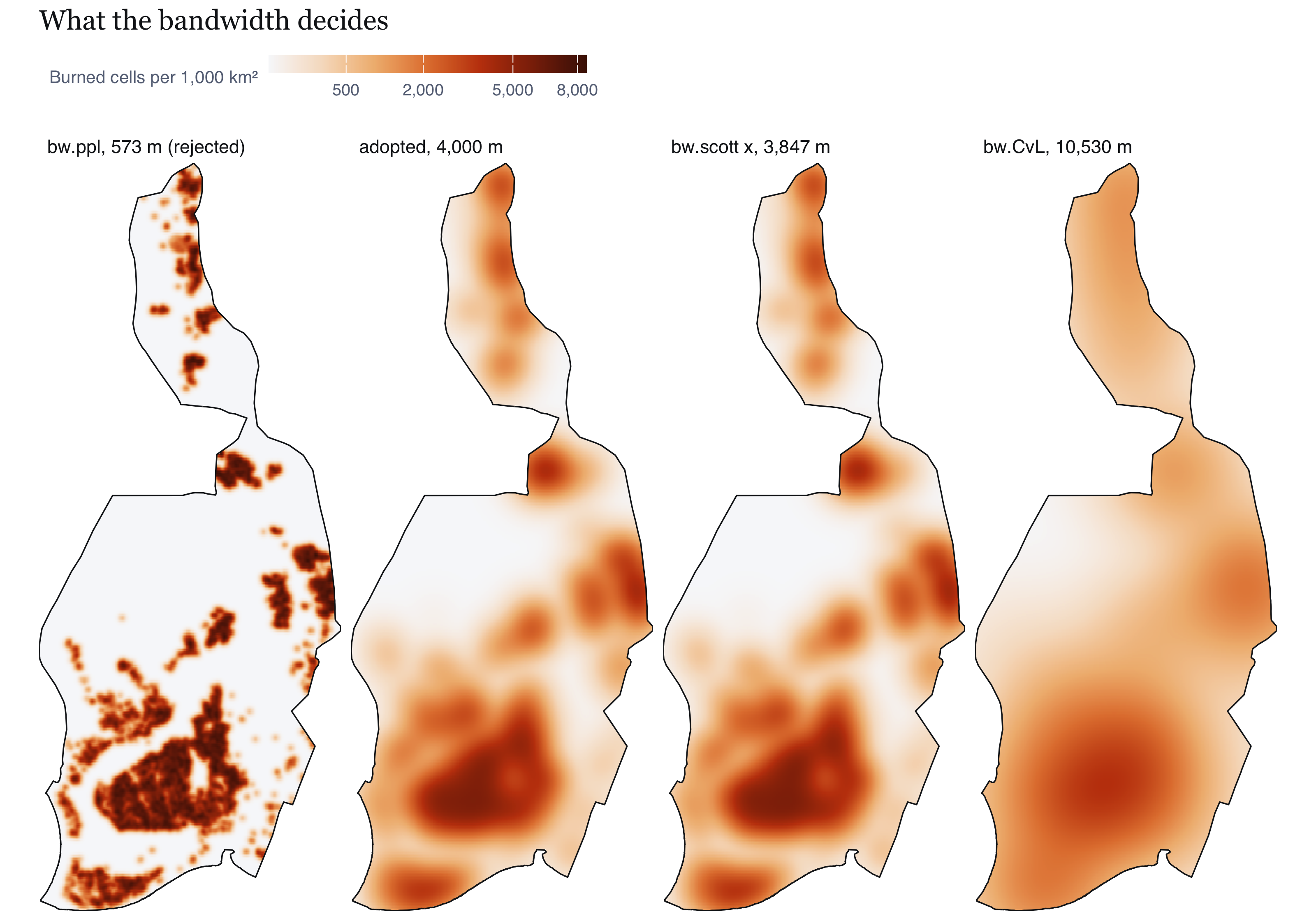
Both cross-validation selectors returned sub-kilometre bandwidths,
`r round(FO$sigma_ppl)` m for `bw.ppl` and `r round(FO$sigma_diggle)` m for
`bw.diggle`, and `density.ppp` threw a numerical-underflow warning at that scale over
a `r fmt_n(round(P$area_km2))` km² window. Neither was adopted, and not because of
the warning.
Cross-validation selectors choose very small bandwidths when a pattern is strongly
clustered at short range. Their criteria reward a surface that reproduces the local
bursts, so clustering gets absorbed into the intensity estimate. For some purposes
that is what you want. Not here. The same estimate becomes the reference intensity
for the second-order test in @sec-honest-test, and if $\hat{\lambda}(u)$ has already
soaked up the sub-kilometre clustering then asking whether clustering survives its
removal is rigged. The answer would be no by construction, and confidently wrong.
So I fixed the bandwidth at **`r fmt_n(FO$sigma_main)` m**, on a criterion I set
before looking at the surfaces: it has to exceed the interaction range, so that
trend and interaction are estimated by separate parts of my analysis instead of
competing for the same signal. Four kilometres sits above the interaction range @sec-second-order goes on to find, inside the interval spanned by the two components of
`bw.scott` (`r fmt_n(round(FO$sigma_scott[1]))` m and
`r fmt_n(round(FO$sigma_scott[2]))` m), and below `bw.CvL`
(`r fmt_n(round(FO$sigma_CvL))` m).
I want to be clear that this is a judgement and not an optimisation. The comparison
below shows what each alternative would have given me, so anyone who disagrees can
see the consequence rather than taking my word for it.
```{r fig-bw}
#| label: fig-bw
#| fig-cap: "The same pattern under four bandwidths. What I take from it: the choice is not cosmetic. The cross-validated surface resolves individual fire complexes and, at this sample size, a great deal of structure no agency could act on; it is also the surface that would sabotage the second-order test, for the reason given above. The 10.5 km bw.CvL surface is stable but has smoothed away the distinction between the peat belt and its margins, which is the distinction of interest. The adopted 4 km surface and bw.scott's 3.8 km are visually close, which is reassurance that the adopted value is not an idiosyncratic pick. What I should disclose is that all four agree on where the principal concentration is and disagree on how many secondary ones exist, so I make no claim about secondary hotspots."
#| fig-height: 5.6
bw_panels <- list(
  ppl   = glue("bw.ppl, {round(FO$sigma_ppl)} m (rejected)"),
  main  = glue("adopted, {fmt_n(FO$sigma_main)} m"),
  scott = glue("bw.scott x, {fmt_n(round(FO$sigma_scott[1]))} m"),
  CvL   = glue("bw.CvL, {fmt_n(round(FO$sigma_CvL))} m"))
bw_df <- bind_rows(lapply(names(bw_panels), function(k)
  im_df(FO$kde[[k]]) |> mutate(panel = bw_panels[[k]]))) |>
  mutate(v = per_1000km2(intensity))
bw_df$panel <- factor(bw_df$panel, levels = unlist(bw_panels))
ggplot(bw_df) +
  geom_raster(aes(x, y, fill = v)) +
  geom_sf(data = win_p, fill = NA, colour = PAL$ink, linewidth = 0.3) +
  facet_wrap(~panel, nrow = 1) +
  scale_fill_intensity(v = bw_df$v) +
  coord_sf(datum = NA, expand = FALSE) +
  labs(title = "What the bandwidth decides") +
  theme_map(base_size = 9)
```
## The intensity surface I report {#sec-intensity}
```{r fig-kde}
#| label: fig-kde
#| fig-width: 6.2
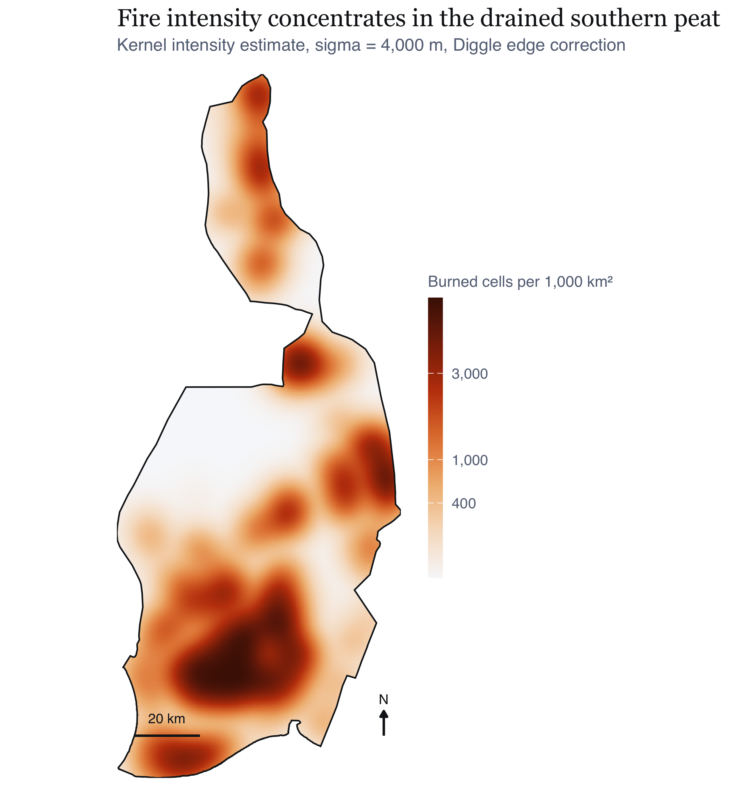
#| fig-cap: "Estimated first-order intensity of burned cells, Gaussian kernel with Diggle's edge correction, at the adopted 4 km bandwidth. What I take from it: intensity is organised as a broad south-southeast band reaching a maximum in the lower third of the regency, with a secondary extension along the eastern margin. The empty northern interior is a real absence rather than an absence of observation: the same satellites observed it on the same days. The gradient is steep, spanning roughly two orders of magnitude between the peat belt and the northern interior, which means resource allocation proportional to intensity would be very unevenly distributed. That is the operational content of a first-order surface, and it is the strongest planning-relevant thing my first-order analysis alone supports."
#| fig-height: 6.6
kde_main <- im_df(FO$kde$main) |> mutate(v = per_1000km2(intensity))
ggplot(kde_main) +
  geom_raster(aes(x, y, fill = v)) +
  geom_sf(data = win_p, fill = NA, colour = PAL$ink, linewidth = 0.45) +
  scale_fill_intensity(v = kde_main$v) +
  coord_sf(datum = NA, expand = FALSE) +
  scalebar_layer(bb) + north_layer(bb) +
  labs(title = "Fire intensity concentrates in the drained southern peat",
       subtitle = glue("Kernel intensity estimate, sigma = {fmt_n(FO$sigma_main)} m, Diggle edge correction")) +
  theme_map() + theme(legend.position = "right", legend.key.height = unit(34, "pt"),
                      legend.key.width = unit(9, "pt"))
```
I also computed an adaptive estimator as a check, because a fixed bandwidth
over-smooths sparse areas and under-smooths dense ones. It reproduces the same
principal concentration, which is the reassurance I was after: the structure I
report is not an artefact of forcing one bandwidth everywhere.
## Radiative power, not just counts
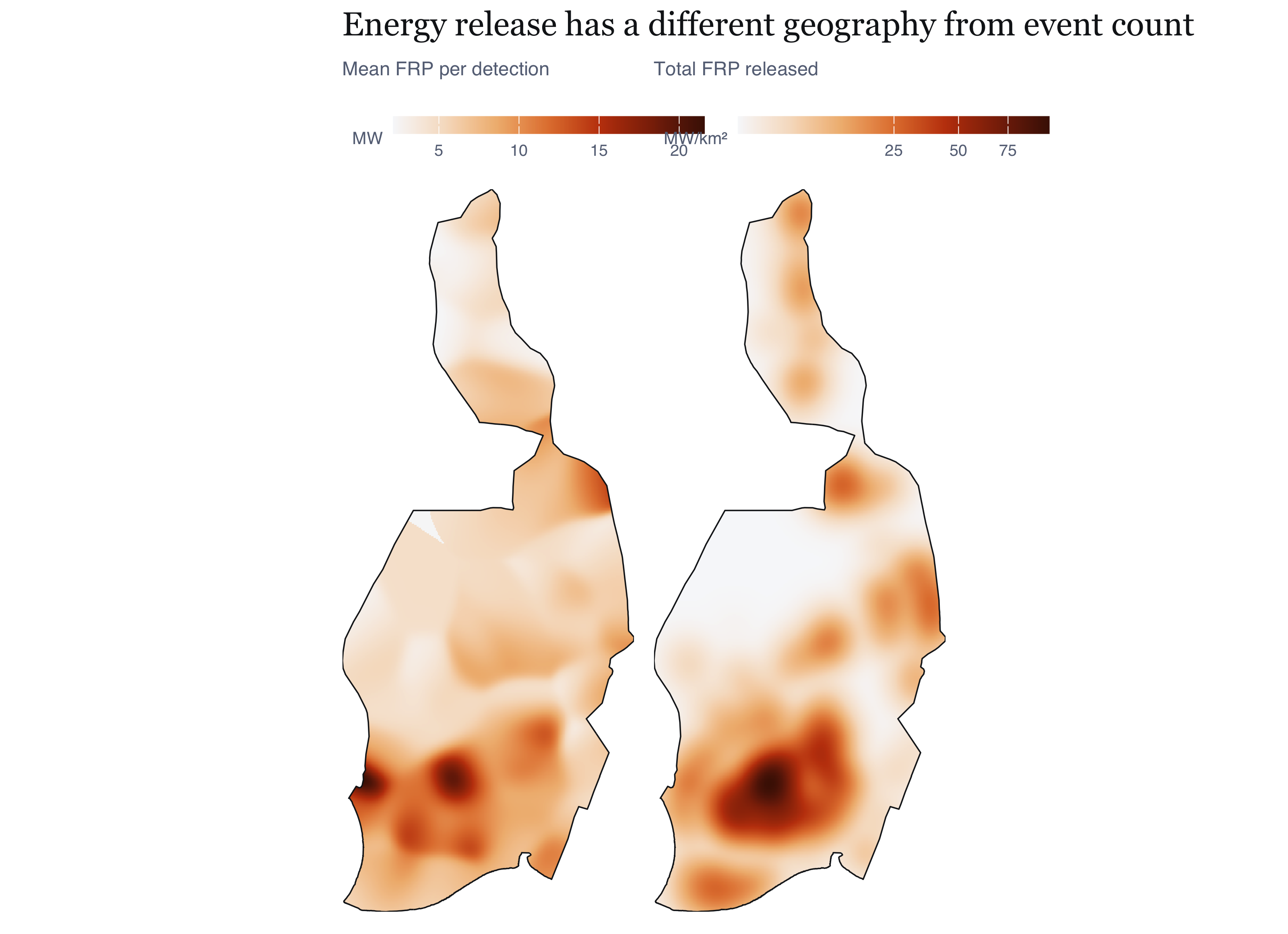
A count surface treats a barely detectable smouldering pixel and an intense flaming
front as the same event, which bothered me. Fire radiative power is the sensor's
estimate of radiative output in megawatts, so smoothing that instead answers a
different and arguably more useful question.
```{r fig-frp}
#| label: fig-frp
#| fig-cap: "Left, mean fire radiative power per detection. Right, total radiative power released, which is intensity and mean power combined. What I take from it: the two panels separate two things a single count map conflates. Total power (right) closely tracks detection intensity, so the southern peat belt dominates energy release as well as event count. Mean power per detection (left) has a different geography: it is comparatively low across the core of the peat belt and higher on the margins and in the sparse north. That is consistent with the physical expectation that peat combustion is low-intensity and persistent while fires on mineral soil and in cleared vegetation burn hotter and shorter. It is also a caution to me: the places with the most detections are not the places with the most intense individual fires."
#| fig-height: 5.8
frp_df  <- im_df(FO$frp_smooth, "v") |> mutate(panel = "Mean FRP per detection (MW)")
frpt_df <- im_df(FO$frp_total, "v") |> mutate(v = v * 1e6, panel = "Total FRP released (MW per km²)")
p1 <- ggplot(frp_df) + geom_raster(aes(x, y, fill = v)) +
  geom_sf(data = win_p, fill = NA, colour = PAL$ink, linewidth = 0.3) +
  scale_fill_gradientn(colours = PAL$seq, name = "MW") +
  coord_sf(datum = NA, expand = FALSE) + labs(subtitle = "Mean FRP per detection") + theme_map(9)
p2 <- ggplot(frpt_df) + geom_raster(aes(x, y, fill = v)) +
  geom_sf(data = win_p, fill = NA, colour = PAL$ink, linewidth = 0.3) +
  scale_fill_gradientn(colours = PAL$seq, trans = "sqrt", name = "MW/km\u00b2",
                       labels = label_number(big.mark = ",")) +
  coord_sf(datum = NA, expand = FALSE) + labs(subtitle = "Total FRP released") + theme_map(9)
p1 + p2 + plot_annotation(title = "Energy release has a different geography from event count",
                          theme = theme_ex01())
```
## Temporal intensity
```{r fig-daily}
#| label: fig-daily
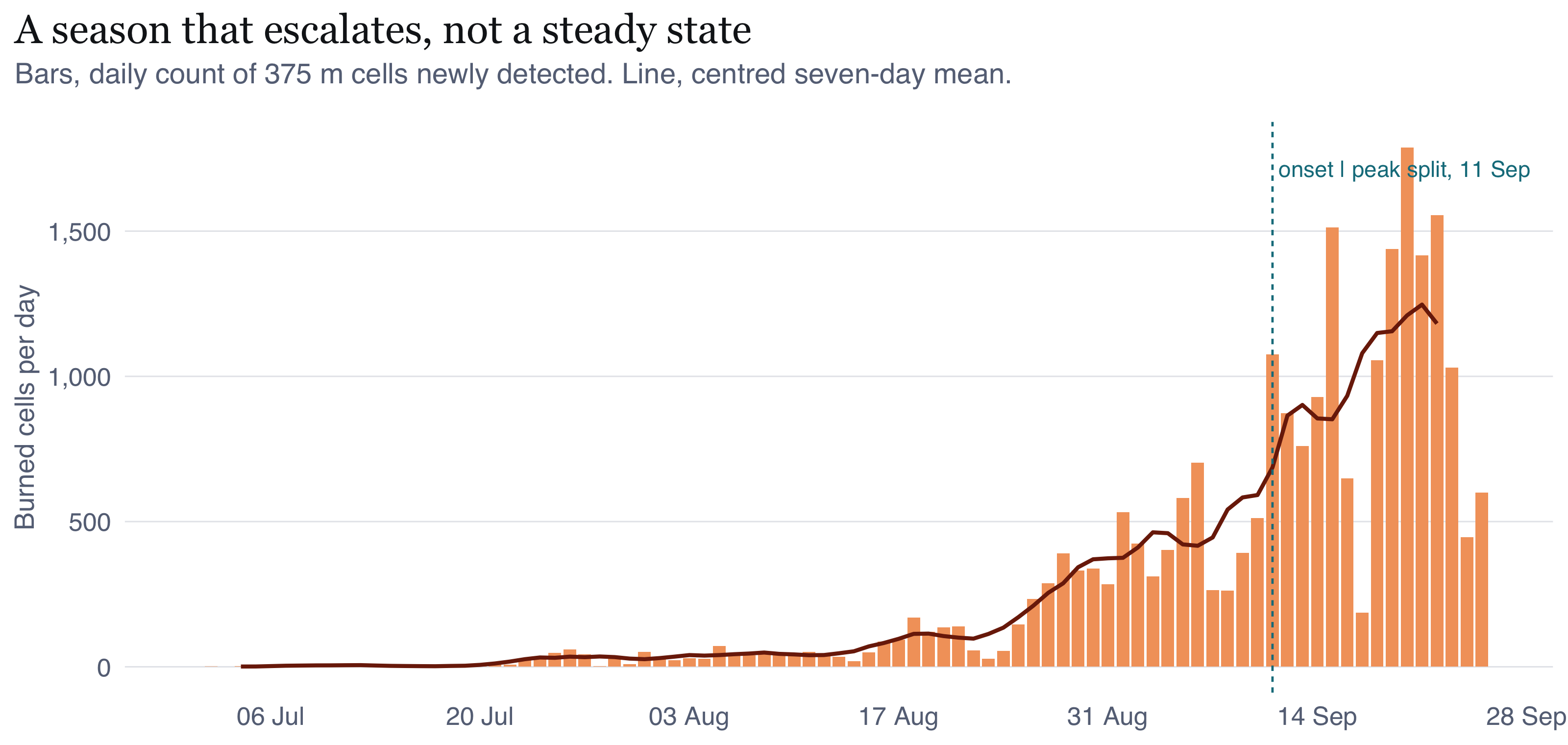
#| fig-cap: "Daily count of burned cells with a centred seven-day mean, and the onset/peak split used later. What I take from it: the episode is not a plateau. Activity is negligible through early July, rises from late July, and escalates sharply through August to a maximum in the first half of September. The seven-day mean is shown because the raw series carries strong short-period structure from cloud cover and overpass geometry, not from fire: a single overcast day suppresses detection regardless of what is burning. I placed the split date by a rule I set in advance, the first day the seven-day mean reaches half its eventual maximum, rather than choosing it after seeing the surfaces I later use it to compare."
#| fig-height: 3.8
dsplit <- ST$split_date
ggplot(FO$daily, aes(date_local)) +
  geom_col(aes(y = n_events), fill = PAL$accent_lt, width = 0.85) +
  geom_line(aes(y = roll7), colour = PAL$accent_dk, linewidth = 0.7) +
  geom_vline(xintercept = as.numeric(dsplit), colour = PAL$cool,
             linetype = "22", linewidth = 0.4) +
  annotate("text", x = dsplit, y = max(FO$daily$n_events) * 0.96,
           label = glue(" onset | peak split, {format(dsplit, '%d %b')}"),
           hjust = 0, size = 2.9, colour = PAL$cool, family = "Helvetica") +
  scale_x_date(date_breaks = "2 weeks", date_labels = "%d %b") +
  scale_y_continuous(labels = label_number(big.mark = ",")) +
  labs(x = NULL, y = "Burned cells per day",
       title = "A season that escalates, not a steady state",
       subtitle = "Bars, daily count of 375 m cells newly detected. Line, centred seven-day mean.") +
  theme_ex01()
```
```{r fig-overpass}
#| label: fig-overpass
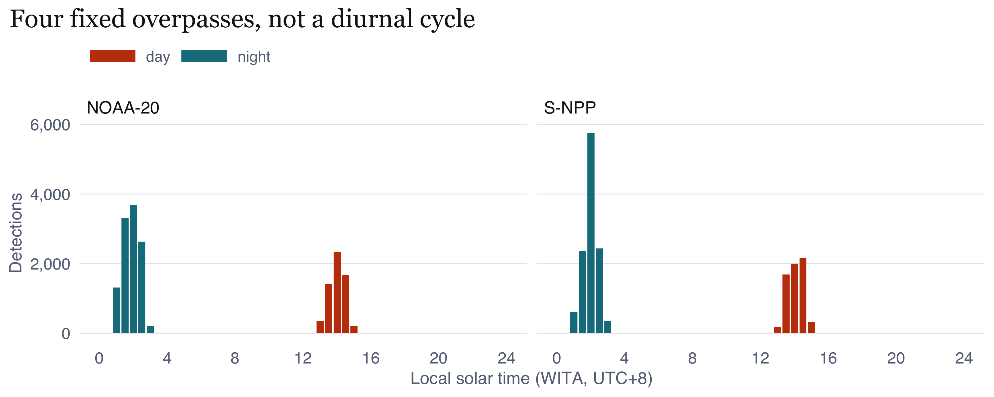
#| fig-cap: "Detections by local solar time of acquisition, split by platform. What I take from it: I put this figure in to stop myself making a mistake. The two platforms observe at four narrow fixed local times, so the apparent day and night counts are not a diurnal cycle of fire activity; they are two sampling windows. Peat fires smoulder continuously and their true diurnal variation cannot be recovered from these data at all. If I said 'fires peak in the early afternoon' I would be describing the satellite's orbit, not the fires. I use the day and night split only as a detectability covariate, since night overpasses catch cooler anomalies against a cooler background."
#| fig-height: 3.2
ggplot(FO$overpass, aes(hr_bin, n, fill = daynight)) +
  geom_col(width = 0.42) +
  facet_wrap(~platform, ncol = 2) +
  scale_fill_manual(values = c(day = PAL$accent, night = PAL$cool), name = NULL) +
  scale_x_continuous(breaks = seq(0, 24, 4), limits = c(0, 24)) +
  scale_y_continuous(labels = label_number(big.mark = ",")) +
  labs(x = "Local solar time (WITA, UTC+8)", y = "Detections",
       title = "Four fixed overpasses, not a diurnal cycle") +
  theme_ex01()
```
# Second-order analysis: clustering, inhibition, or randomness {#sec-second-order}
## The straw man I had to test anyway {#sec-strawman}
```{r fig-csr}
#| label: fig-csr
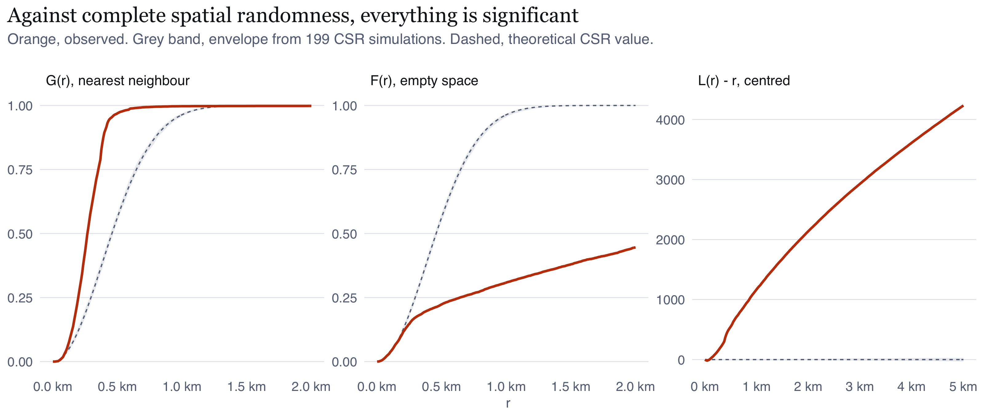
#| fig-cap: "Nearest-neighbour G, empty-space F, and the centred L function, each against a complete spatial randomness envelope from 199 simulations. What I take from it: every statistic departs from the CSR envelope immediately and by an enormous margin. G rises far faster than expected, meaning nearest neighbours are much closer than random; F rises far slower, meaning empty gaps are much larger than random; L sits far above zero at every lag. Read naively this is overwhelming evidence of clustering. Read correctly it is evidence of almost nothing, because the sensor guarantees this result: a single fire produces adjacent detections. I include it to make that failure visible rather than hide it. The analysis I actually rely on is in Section 7.3."
#| fig-height: 3.4
mk_env_df <- function(e, lab) e |> mutate(panel = lab)
eg <- mk_env_df(SO$env_G, "G(r), nearest neighbour")
ef <- mk_env_df(SO$env_F, "F(r), empty space")
el <- SO$env_L |>
  mutate(across(c(obs, theo, lo, hi), ~ .x - r), panel = "L(r) - r, centred")
env_all <- bind_rows(eg, ef, el)
env_all$panel <- factor(env_all$panel, levels = c("G(r), nearest neighbour",
                                                  "F(r), empty space", "L(r) - r, centred"))
ggplot(env_all, aes(r)) +
  geom_ribbon(aes(ymin = lo, ymax = hi), fill = PAL$rule, alpha = 0.75) +
  geom_line(aes(y = theo), colour = PAL$muted, linetype = "22", linewidth = 0.35) +
  geom_line(aes(y = obs), colour = PAL$accent, linewidth = 0.7) +
  facet_wrap(~panel, scales = "free", nrow = 1) +
  scale_x_continuous(labels = label_number(scale = 1e-3, suffix = " km")) +
  labs(x = "r", y = NULL,
       title = "Against complete spatial randomness, everything is significant",
       subtitle = glue("Orange, observed. Grey band, envelope from {SO$nsim} CSR simulations. Dashed, theoretical CSR value.")) +
  theme_ex01(base_size = 9)
```
## What the pair correlation function reveals about the instrument
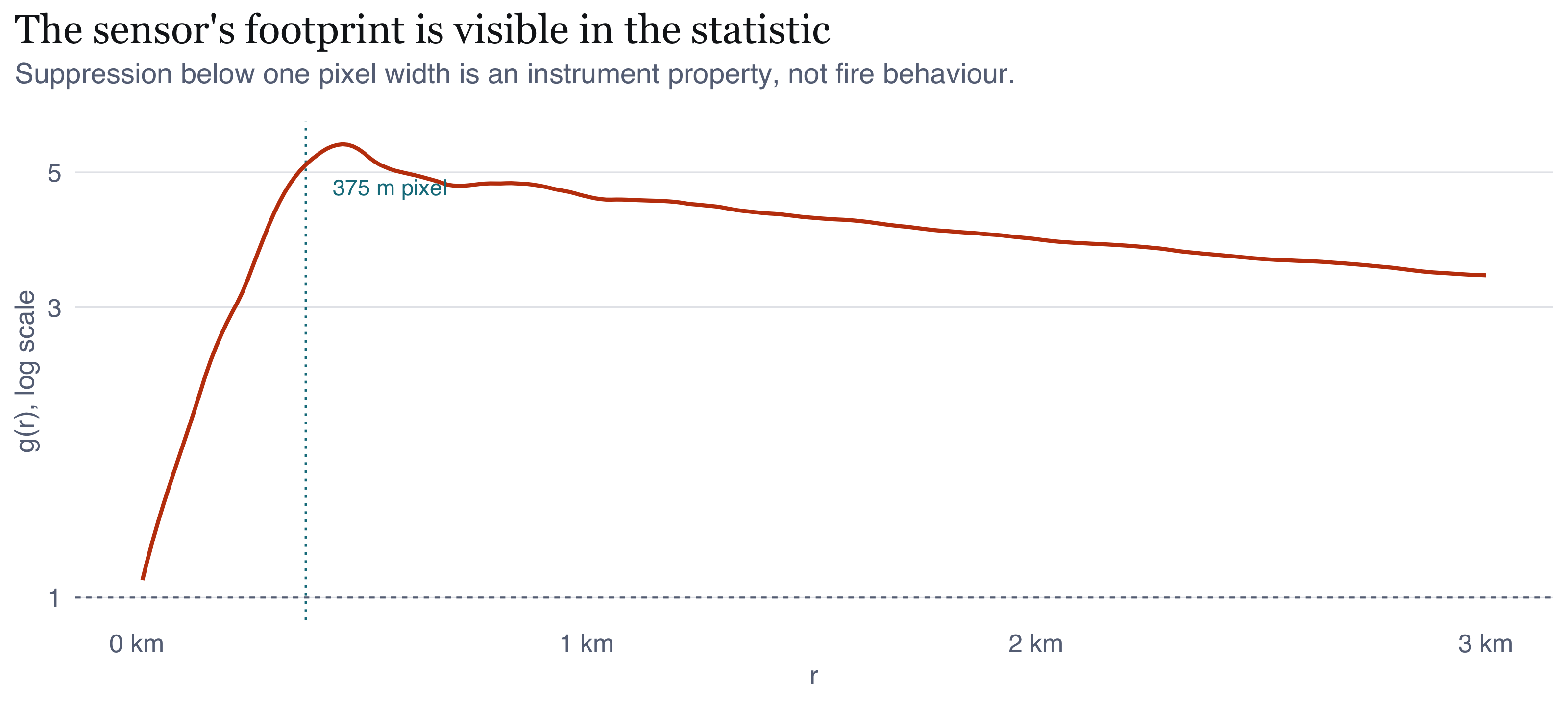
$K$ and $L$ are cumulative, so a departure at one lag propagates into every larger
one and the location of the effect is invisible. The pair correlation function
$g(r)$ is a density, and it separates scales. That distinction matters more here
than I expected.
```{r fig-pcf}
#| label: fig-pcf
#| fig-cap: "Pair correlation function of the primary pattern, log scale. The dotted line marks the 375 m VIIRS pixel dimension. What I take from it: g(r) is suppressed at very short range and peaks at about 460 m, immediately above the pixel width. This is not fires avoiding one another. It is the sensor's resolution: two detections cannot be much closer than one pixel, because one pixel yields one detection. That short-range suppression is an instrument artefact and is the clearest single piece of evidence that this pattern records observation rather than events. Above the peak, g(r) decays slowly and is still above 3 at 2.9 km, nowhere near its asymptote of 1. So spatial dependence extends well beyond the 5 km range I plot here, which is what pushed me to the extended range in Section 7.6."
#| fig-height: 3.6
pcf_df <- SO$pcf_obs |> filter(is.finite(trans), r > 0)
ggplot(pcf_df, aes(r, trans)) +
  geom_hline(yintercept = 1, colour = PAL$muted, linetype = "22", linewidth = 0.35) +
  geom_vline(xintercept = DEDUP_GRID_M, colour = PAL$cool, linetype = "12", linewidth = 0.4) +
  geom_line(colour = PAL$accent, linewidth = 0.7) +
  annotate("text", x = DEDUP_GRID_M + 60, y = max(pcf_df$trans) * 0.85,
           label = "375 m pixel", hjust = 0, size = 2.9, colour = PAL$cool,
           family = "Helvetica") +
  scale_x_continuous(labels = label_number(scale = 1e-3, suffix = " km")) +
  scale_y_log10() +
  labs(x = "r", y = "g(r), log scale",
       title = "The sensor's footprint is visible in the statistic",
       subtitle = "Suppression below one pixel width is an instrument property, not fire behaviour.") +
  theme_ex01()
```
## The test that can fail {#sec-honest-test}
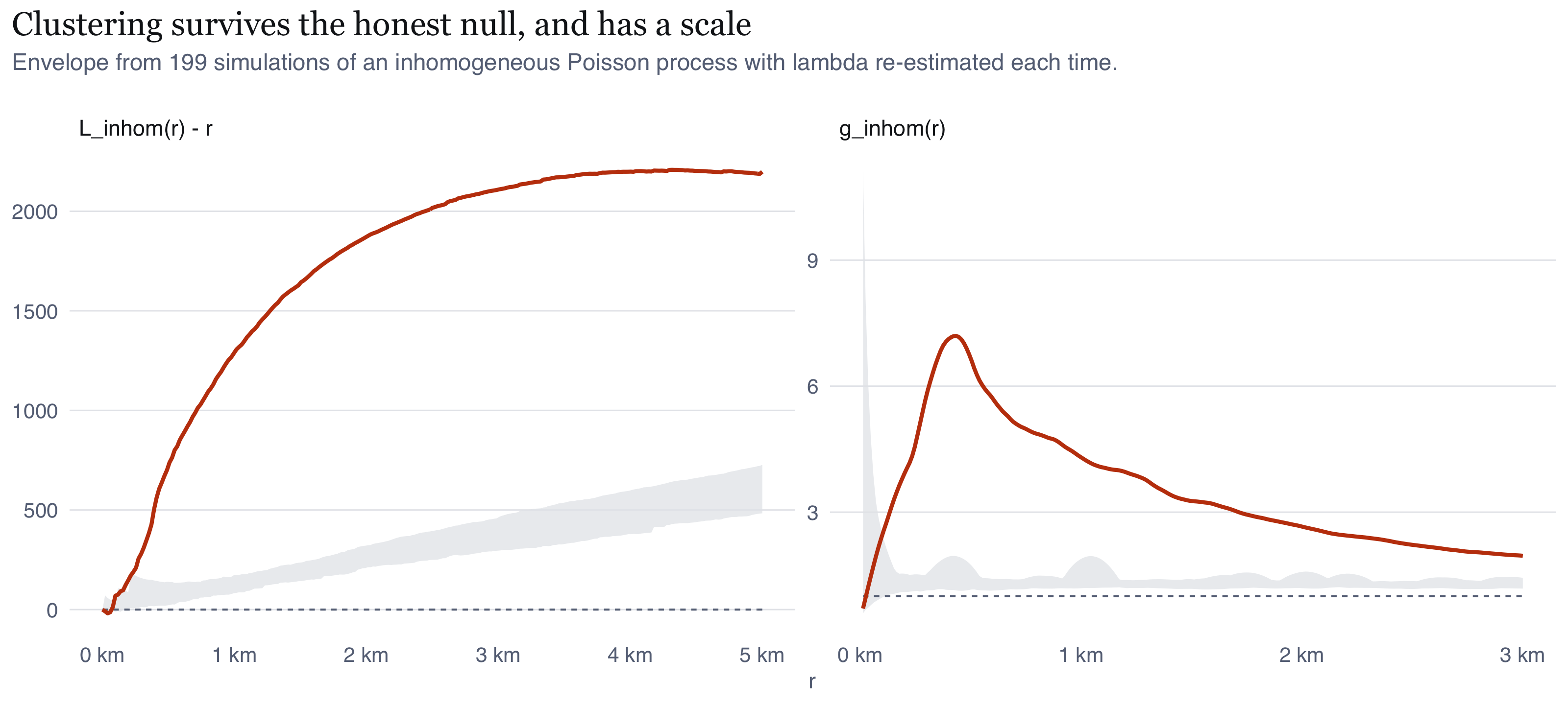
These are the statistics I trust. The null is an inhomogeneous Poisson process
whose intensity is the kernel estimate from @sec-intensity, so everything the
first-order analysis established sits inside the null already. A departure now means
residual interaction, not large-scale variation. That is Q3.
```{r fig-inhom}
#| label: fig-inhom
#| fig-cap: "Inhomogeneous centred L function and inhomogeneous pair correlation function, against envelopes from 199 simulations of an inhomogeneous Poisson process. The reference intensity is re-estimated for every simulated pattern. What I take from it: the departure survives, and it does not close. Both curves leave the envelope at about 100 m and remain outside it across the entire range plotted. g_inhom peaks near 5.9 at roughly 570 m and is still above 2 at 2.8 km, against an envelope ceiling near 1.4. So after accounting for the fact that fire is far more likely in the southern peat belt than in the north, burned cells still occur much closer together than that variation alone predicts. Note also that g_inhom falls below 1 at the shortest lags, the sensor floor surviving into the inhomogeneous statistic."
#| fig-height: 3.6
# An envelope built from `simulate=` has no theoretical curve, only the simulation
# mean, so the reference is set explicitly: 0 for the centred L function and 1 for
# the pair correlation function.
li <- SO$env_Linhom |> mutate(across(c(obs, lo, hi), ~ .x - r),
                              ref = 0, panel = "L_inhom(r) - r")
gi <- SO$env_pcfinhom |> filter(r > 0) |> mutate(ref = 1, panel = "g_inhom(r)")
ggplot(bind_rows(li, gi), aes(r)) +
  geom_ribbon(aes(ymin = lo, ymax = hi), fill = PAL$rule, alpha = 0.75) +
  geom_line(aes(y = ref), colour = PAL$muted, linetype = "22", linewidth = 0.35) +
  geom_line(aes(y = obs), colour = PAL$accent, linewidth = 0.7) +
  facet_wrap(~panel, scales = "free", nrow = 1) +
  scale_x_continuous(labels = label_number(scale = 1e-3, suffix = " km")) +
  labs(x = "r", y = NULL,
       title = "Clustering survives the honest null, and has a scale",
       subtitle = glue("Envelope from {SO$nsim} simulations of an inhomogeneous Poisson process with lambda re-estimated each time.")) +
  theme_ex01(base_size = 9)
```
```{r tbl-global}
#| label: tbl-global
#| tbl-cap: "Global Monte Carlo tests. The maximum absolute deviation (MAD) and Diggle-Cressie-Loosmore-Ford (DCLF) statistics each summarise the whole curve in one number, so these p-values are not inflated by reading a band at many lags. The Monte Carlo floor is 0.01 with 99 simulations."
tibble::tribble(
  ~Test, ~Statistic, ~Null, ~`p-value`,
  "MAD",  "L(r)",       "complete spatial randomness",  fmt_p(SO$mad_L$p.value, 99),
  "MAD",  "L_inhom(r)", "inhomogeneous Poisson",        fmt_p(SO$mad_Linhom$p.value, 99),
  "DCLF", "L_inhom(r)", "inhomogeneous Poisson",        fmt_p(SO$dclf_Linhom$p.value, 99)
) |> kable(align = "lllr")
```
Both global tests reject the inhomogeneous Poisson null at the Monte Carlo floor.
The pattern is clustered beyond its first-order trend, which answers the first half
of Q3.
Where the clustering ends is a different matter, and here a decision of mine got in
the way. I capped r at 5 km on the reasoning that longer lags in an elongated window
rest on too few pairs. Across that whole range both curves sit outside the envelope.
All 5 km establishes is that dependence extends *at least* that far. @sec-extended
extends the range.
The direction of the remaining bias matters for how confidently this can be
stated. As set out in assumption A6, estimating $\hat{\lambda}$ from the pattern
under test lets it absorb part of the clustering, which widens the envelope and
makes the test *harder* to reject. The rejection therefore stands despite a
conservative procedure, not because of a permissive one.
## Testing isotropy, instead of just assuming it {#sec-isotropy}
Assumption A7 says $K$, $L$ and $g$ all average over direction, and that I expected
real anisotropy because peat fires spread with the wind and along canal lines.
Listing an assumption and never testing it is the kind of thing that should not
survive a read, so this section tests it. The test found something, but not the
thing I predicted, and the first version of my own analysis missed it.
**Why I did not use the packaged tools.** `spatstat` offers `Ksector` and
`pairorient`, and neither accepts a `lambda` argument: both assume homogeneity.
Applied here they would reject isotropy for two reasons that have nothing to do
with fire. The window is 86 km wide and 213 km tall, so even a perfectly isotropic
process yields more north-south pairs than east-west ones purely because there is
more room that way. And intensity is concentrated in a south-southeast band, so any
pair drawn from inside it inherits that elongation.
I therefore built the null the way I built it for clustering: simulate from an
inhomogeneous Poisson process with the same $\hat{\lambda}$ from @sec-first-order, which
absorbs the window geometry and the first-order trend together.
**Two statistics, and the second one is the point.** Orientations here are axial, so
I double the angles before averaging and summarise concentration by the mean
resultant length $R_2 = |n^{-1}\sum_k e^{2i\theta_k}|$, which is 0 when
orientations are spread evenly and 1 when every pair lies on one axis.
Each harmonic is blind to the next one up, and I walked into that twice.
$R_2$ detects a single preferred axis and is **structurally blind to four-fold
structure**, because a rose with spikes at 0 and 90 degrees has its doubled angles
cancel. My first version of this section reported the short range as isotropic on
the strength of $R_2$ alone, and the rose diagram contradicted it on sight. So I
added $R_4 = |n^{-1}\sum_k e^{4i\theta_k}|$.
$R_4$ is in turn blind to **eight-fold** structure. Spikes at 0, 45, 90 and 135
degrees have a 45-degree period, so under $e^{4i\theta}$ the 45 and 135 pair sits
in antiphase to the 0 and 90 pair and the two cancel. That is exactly the shape a
square grid produces, because a lattice offers displacements along its axes *and*
along its diagonals. $R_8$ is what captures it, and it turns out to be the largest
directional signal anywhere in this analysis.
A harmonic statistic finds only the structure you asked it about. Two passes were
needed here because I kept asking the wrong one, and each time the rose diagram was
what showed me.
```{r tbl-aniso}
#| label: tbl-aniso
#| tbl-cap: "Directional structure by distance band against 199 simulations of an inhomogeneous Poisson process in the same window. R2 detects a single preferred axis, R4 four-fold structure, R8 eight-fold. Note that at 375 to 750 m the three disagree completely: R2 sees nothing, R4 sees something, and R8 sees the largest effect in the whole analysis."
AN$results |> transmute(
  Band = glue("{r1} to {r2} m"),
  Pairs = fmt_n(n_pairs),
  `R2` = round(R_obs, 4), `p R2` = vapply(p_resultant, fmt_p, character(1), nperm = AN$nsim),
  `R4` = round(R4_obs, 4), `p R4` = vapply(p_fourfold, fmt_p, character(1), nperm = AN$nsim),
  `R8` = round(R8_obs, 4), `p R8` = vapply(p_eightfold, fmt_p, character(1), nperm = AN$nsim),
  `null R8` = round(R8_null_mean, 4)
) |> kable(align = "lrrrrrrrr")
```
```{r fig-aniso}
#| label: fig-aniso
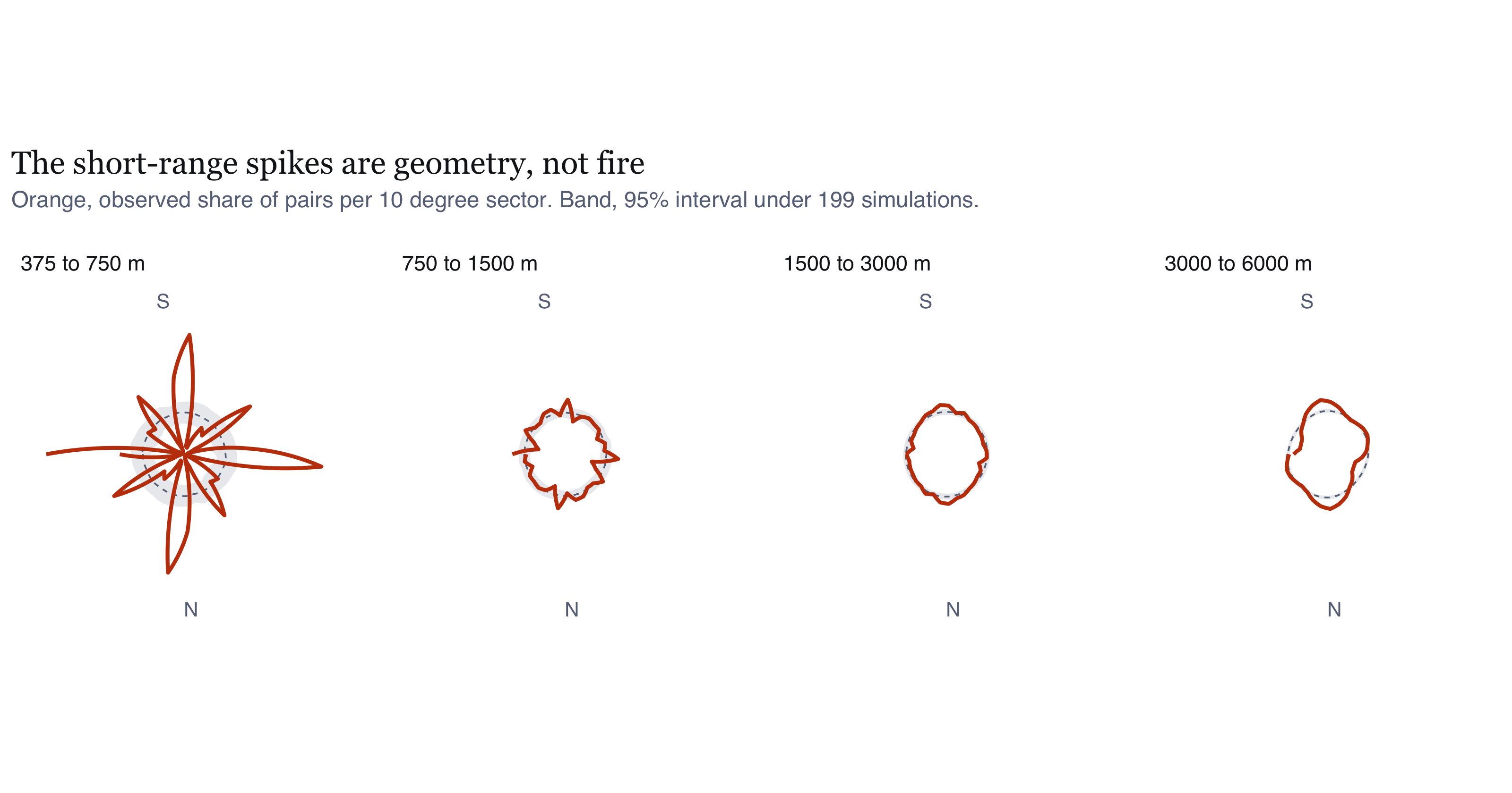
#| fig-cap: "Orientation of close pairs by distance band, as a rose diagram, against the 95% interval from 199 inhomogeneous Poisson simulations. Each rose is mirrored across the origin because orientations are axial. What I take from it: the shortest band is not isotropic at all. It has eight sharp spikes on the cardinal axes and the diagonals, which is the signature of a square grid rather than of fire, and my R2 statistic scored it as isotropic because R2 cannot see four-fold structure. The figure caught what the table missed. From 750 m outward the spikes vanish and the roses sit close to their null intervals, with only a slight and growing elongation by 3 to 6 km."
#| fig-height: 4.2
rose <- AN$results |> select(r1, r2, props) |> tidyr::unnest(props) |>
  mutate(band = factor(glue("{r1} to {r2} m"),
                       levels = glue("{AN$results$r1} to {AN$results$r2} m")))
rose2 <- bind_rows(rose, rose |> mutate(lo_deg = lo_deg + 180))
ggplot(rose2, aes(lo_deg)) +
  geom_ribbon(aes(ymin = null_lo, ymax = null_hi, group = band),
              fill = PAL$rule, alpha = 0.8) +
  geom_line(aes(y = null, group = band), colour = PAL$muted,
            linetype = "22", linewidth = 0.3) +
  geom_line(aes(y = obs, group = band), colour = PAL$accent, linewidth = 0.7) +
  coord_polar(start = pi/2, direction = -1) +
  facet_wrap(~band, nrow = 1) +
  # Only N and S are labelled. With four polar facets side by side, an E on one
  # panel sits directly against the W of the next and the two read as one word.
  scale_x_continuous(breaks = c(90, 270), labels = c("N", "S")) +
  scale_y_continuous(labels = NULL, name = NULL) +
  labs(x = NULL,
       title = "The short-range spikes are geometry, not fire",
       subtitle = glue("Orange, observed share of pairs per 10 degree sector. Band, 95% interval under {AN$nsim} simulations.")) +
  theme_ex01(base_size = 9, grid = "none") +
  theme(axis.text.y = element_blank(),
        panel.spacing = unit(14, "pt"))
```
```{r}
#| label: aniso-inline
#| include: false
a_short <- AN$results |> filter(r1 == 375)
a_mid <- AN$results |> filter(r1 == 750)
a_long <- AN$results |> filter(r1 == 3000)
wat <- AN$networks |> filter(network == "waterways")
rds <- AN$networks |> filter(network == "roads")
ctl_cell <- AN$control |> filter(grepl("ppp_cell", pattern))
ctl_all <- AN$control |> filter(grepl("ppp_all", pattern))
axsep <- function(a, b) { d <- abs(a - b) %% 180; pmin(d, 180 - d) }
```
### The short-range structure is my grid, and the sensor's
Over `r a_short$r1` to `r a_short$r2` m the eight-fold concentration is
`r round(a_short$R8_obs, 4)` against `r round(a_short$R8_null_mean, 4)` under the
null, `r fmt_p(a_short$p_eightfold, AN$nsim)`. That is more than twelve times the
null value and the largest directional effect measured anywhere in this report. The
four-fold term is `r round(a_short$R4_obs, 4)`, also significant, and $R_2$ is
`r round(a_short$R_obs, 4)` against a null of `r round(a_short$R_null_mean, 4)`,
`r fmt_p(a_short$p_resultant, AN$nsim)`, which is nothing at all.
Three statistics on the same 36,860 pairs, and they disagree completely. The
structure is spikes on the axes and on the diagonals, which is what a square
lattice produces and what only the eighth harmonic can see.
My first explanation was that this is entirely my own doing. `ppp_cell` keeps at
most one point per 375 m cell, so short-range displacements are dominated by
lattice vectors: 375 m at 0 and 90 degrees, 530 m on the diagonals, 750 m at two
cells. That would produce spikes exactly where they appear. The way to check it is
to run the identical test on `ppp_all`, which keeps every detection at its own
sensor coordinate and has no such lattice.
```{r tbl-aniso-control}
#| label: tbl-aniso-control
#| tbl-cap: "The same test over 375 to 750 m, on the thinned pattern and on the un-thinned detections. If the spikes were purely an artefact of my cell thinning, the second row would show nothing. It does not."
AN$control |> transmute(
  Pattern = pattern, n = fmt_n(n), Pairs = fmt_n(n_pairs),
  `R8 obs` = round(R8_obs, 4), `R8 null` = round(R8_null, 4),
  `p R8` = vapply(p_eightfold, fmt_p, character(1), nperm = AN$nsim_control),
  `R4 obs` = round(R4_obs, 4),
  `p R4` = vapply(p_fourfold, fmt_p, character(1), nperm = AN$nsim_control)
) |> kable(align = "lrrrrrrr")
```
The control only half-confirms my explanation, which is more interesting than if it
had confirmed it outright. Thinning multiplies the eight-fold signal by about two
and a half, from `r round(ctl_all$R8_obs, 4)` to `r round(ctl_cell$R8_obs, 4)`, so
a large part of the structure is indeed my construction. But the un-thinned
detections still show `r round(ctl_all$R8_obs, 4)` against a null of
`r round(ctl_all$R8_null, 4)`, `r fmt_p(ctl_all$p_eightfold, AN$nsim_control)`,
which is roughly nineteen times the null. Removing my lattice reduces the effect
without removing it.
The remainder is the instrument. VIIRS reports detections on its own scan grid,
organised along-scan and along-track, and for a polar orbiter those project to
roughly cardinal directions on the ground. So the raw detections carry a
quasi-rectangular sampling geometry before I do anything to them.
Neither component is fire. Both are instrument geometry, which is the warning from @sec-not-a-fire applied to my own directional test.
### At longer range, a real but negligible tilt
From 750 m outward every harmonic goes quiet. Over
`r a_mid$r1` to `r a_mid$r2` m, $R_4$ is `r round(a_mid$R4_obs, 4)`
(`r fmt_p(a_mid$p_fourfold, AN$nsim)`) and $R_8$ is `r round(a_mid$R8_obs, 4)`
(`r fmt_p(a_mid$p_eightfold, AN$nsim)`), both below their nulls. That is what a
lattice explanation predicts, since every lattice vector is shorter than 750 m, and
it is the check that makes me believe the short-range result is geometric rather
than physical.
What remains is a weak single-axis elongation that grows with distance, reaching
$R_2 =$ `r round(a_long$R_obs, 4)` over `r a_long$r1` to `r a_long$r2` m against a
null of `r round(a_long$R_null_mean, 4)`. That is statistically distinguishable at
the Monte Carlo floor and it is 2.4% of the way to perfect alignment, which is not
a directional pattern in any sense a fire officer would recognise.
### My stated mechanism was wrong
A7 guessed that fires would align with canal lines. They do not.
```{r tbl-aniso-net}
#| label: tbl-aniso-net
#| tbl-cap: "Orientation of the mapped drainage and road networks inside the regency, weighted by segment length, against the fire pair-orientation axis at each band. Separation is axial, so 90 degrees is the maximum possible disagreement."
bind_rows(
  AN$networks |> transmute(What = network, `Length (km)` = fmt_n(round(total_km)),
                           R2 = round(R, 4), `Axis (deg)` = round(axis_deg)),
  AN$results |> transmute(What = glue("fire pairs, {r1} to {r2} m"),
                          `Length (km)` = "", R2 = round(R_obs, 4),
                          `Axis (deg)` = round(axis_deg))
) |> kable(align = "lrrr")
```
The mapped waterways run at about `r round(wat$axis_deg)` degrees and the roads at
about `r round(rds$axis_deg)` degrees. The long-range fire axis is
`r round(a_long$axis_deg)` degrees: `r round(axsep(a_long$axis_deg, wat$axis_deg))`
degrees off the drainage and `r round(axsep(a_long$axis_deg, rds$axis_deg))` degrees
off the roads, on a scale where 90 degrees is the maximum possible disagreement.
Neither is a match.
So the weak long-range tilt is not canal-following. It runs closer to north-south,
which is also the long axis of the regency and of the peat belt inside it. The most
likely explanation is first-order structure that $\hat{\lambda}$ at a 4 km
bandwidth does not fully absorb, not a directional process in the fire. I
cannot separate those two with this design and I will not claim otherwise.
### What this changes
A7 said anisotropy was likely because fires follow canals, and that it made my
clustering estimates conservative. Both claims fail.
The short-range structure is geometric. It comes from the 375 m cell grid and the
sensor's scan grid, not from wind or canals. Beyond 750 m, where the clustering
lives, no harmonic finds anything. The isotropic $K$, $L$ and $g$ estimate what they
claim to, and there is no conservatism to claim.
One practical consequence for the rest of the report. Because the eight-fold
structure is symmetric about the cardinal axes and the diagonals, it very largely
cancels in any statistic that averages over direction, which is what $K$, $L$ and
$g$ do. So it does not bias the clustering results. It would wreck a directional
analysis, and anyone extending this work should thin differently before attempting
one.
## Sensitivity to the event definition
My whole analysis rests on collapsing detections to cells, so I wanted to know
whether the finding depends on that choice. If it did, it would be a finding about
my choice rather than about fire.
```{r fig-sens}
#| label: fig-sens
#| fig-cap: "Inhomogeneous centred L function computed on the cell pattern and on the un-thinned detection pattern, on a common axis. What I take from it: both curves are positive, so the qualitative conclusion of residual clustering does not depend on the event definition. The magnitudes differ by roughly an order of magnitude, and the un-thinned pattern shows far stronger apparent clustering at every lag. That gap is the repeat-detection artefact measured directly. It is why I use the cell pattern for inference and the detection pattern only for this check. If I reported the upper curve I would be reporting the satellite revisit schedule as a fire-behaviour result."
#| fig-height: 3.4
sd_df <- bind_rows(
  SO$Linhom_cell |> transmute(r, v = border - r, pattern = "ppp_cell (reported)"),
  SO$Linhom_all  |> transmute(r, v = border - r, pattern = "ppp_all (un-thinned)"))
ggplot(sd_df, aes(r, v, colour = pattern)) +
  geom_hline(yintercept = 0, colour = PAL$muted, linetype = "22", linewidth = 0.35) +
  geom_line(linewidth = 0.7) +
  scale_colour_manual(values = c("ppp_cell (reported)" = PAL$accent,
                                 "ppp_all (un-thinned)" = PAL$cool), name = NULL) +
  scale_x_continuous(labels = label_number(scale = 1e-3, suffix = " km")) +
  labs(x = "r", y = "L_inhom(r) - r",
       title = "The conclusion is robust, the magnitude is not",
       subtitle = glue("n = {fmt_n(SO$n_cell)} cells against n = {fmt_n(SO$n_all)} detections.")) +
  theme_ex01()
```
## Extending the range, after getting it wrong {#sec-extended}
I set the 5 km cap because long lags in an elongated window rest on few pairs. That
reasoning is fine, but 5 km was more conservative than I needed. The rule I stated in @sec-assumptions caps $r$ at a quarter of the window's shortest dimension, and the window is
`r round((bb["xmax"]-bb["xmin"])/1000)` km wide, so 20 km was admissible the whole
time. Extending to 20 km is not me granting myself a post-hoc licence, it is me
finally applying the rule I had already written down.
Two practical constraints came with that, and I am disclosing both rather than
hiding them. `pcfinhom` offers no border correction, and the translation correction
over roughly seven million pairs per pattern would not finish in a workable time for
99 simulated patterns. So my significance across the extended range rests on
$L_{inhom}$ with a border correction and a full envelope, while the shape of
$g_{inhom}$ comes from a single translation-corrected curve with no simulations.
**I make no significance claim for $g_{inhom}$ beyond 3 km.**
```{r fig-ext}
#| label: fig-ext
#| fig-cap: "Left, inhomogeneous centred L function to 20 km with a 99-simulation envelope. Right, the observed inhomogeneous pair correlation function over the same range, with no envelope, on a log scale. What I take from it: the two panels answer different questions and disagree in an instructive way. g_inhom, which localises scale, peaks at about 440 m and decays steadily: it is 4.3 at 1 km, 2.7 at 2 km, 1.4 at 5 km, and reaches within 10% of its asymptote of 1 at about 7.2 km. L_inhom, which is cumulative, never re-enters its envelope within 20 km. Both are correct. The excess pair density is a local phenomenon that has largely dissipated by 7 km, and because L accumulates every excess at smaller lags it remains significantly elevated far beyond the range over which anything is actually happening."
#| fig-height: 3.6
Lx <- EX$env_L_ext |> mutate(across(c(obs, lo, hi), ~ .x - r), ref = 0,
                             panel = "L_inhom(r) - r, with envelope")
Gx <- EX$g_obs_ext |> filter(r > 0, is.finite(trans)) |>
  transmute(r, obs = trans, lo = NA_real_, hi = NA_real_, ref = 1,
            panel = "g_inhom(r), observed only")
ggplot(bind_rows(Lx, Gx), aes(r)) +
  geom_ribbon(aes(ymin = lo, ymax = hi), fill = PAL$rule, alpha = 0.75, na.rm = TRUE) +
  geom_line(aes(y = ref), colour = PAL$muted, linetype = "22", linewidth = 0.35) +
  geom_line(aes(y = obs), colour = PAL$accent, linewidth = 0.7) +
  geom_vline(data = tibble(panel = "g_inhom(r), observed only",
                           x = EX$summary_ext$r_g_within_10pct_of_1),
             aes(xintercept = x), colour = PAL$cool, linetype = "12", linewidth = 0.4) +
  facet_wrap(~panel, scales = "free", nrow = 1) +
  scale_x_continuous(labels = label_number(scale = 1e-3, suffix = " km")) +
  labs(x = "r", y = NULL,
       title = "Dependence is local, but a cumulative statistic cannot say so",
       subtitle = glue("Dotted line marks {round(EX$summary_ext$r_g_within_10pct_of_1/1000, 1)} km, where g_inhom first comes within 10% of 1.")) +
  theme_ex01(base_size = 9)
```
```{r tbl-ext}
#| label: tbl-ext
#| tbl-cap: "Observed inhomogeneous pair correlation at selected lags. A value of 1 means no excess over the inhomogeneous Poisson expectation."
with(EX$summary_ext, tibble::tibble(
  Lag = c("peak", "1 km", "2 km", "5 km", "10 km", "20 km"),
  `g_inhom` = round(c(peak_g, g_1km, g_2km, g_5km, g_10km, g_20km), 2),
  Note = c(glue("at {round(peak_r_m)} m"), "", "", "", "", "sampling noise at this lag")
)) |> kable(align = "lrl")
```
```{r}
#| label: ext-crosscheck
#| include: false
cc <- EX$correction_cmp
cc_med <- 100 * median(abs(cc$rel_diff), na.rm = TRUE)
```
I cross-checked the extended curve against my @sec-honest-test estimate over the lags
both cover, since both use the translation correction. The median relative difference
is `r sprintf("%.2f%%", cc_med)`, so changing the $r$ grid has not quietly changed
the estimate underneath me.
**So here is my corrected answer to Q3.** Residual clustering begins immediately
above the sensor floor, is strongest at roughly
`r round(EX$summary_ext$peak_r_m)` m, and only decays to within 10% of no excess by
about `r round(EX$summary_ext$r_g_within_10pct_of_1/1000, 1)` km. My earlier
statement that the excess was exhausted by 2 km was simply an artefact of not having
looked far enough, and the conclusion I drew from it, that the first-order surface
was a sufficient description above 2 km, was wrong. It is not sufficient at any lag
below roughly 7 km.
# Spatio-temporal analysis {#sec-spacetime}
## Space-time interaction
```{r tbl-knox}
#| label: tbl-knox
#| tbl-cap: "Knox test of space-time interaction across a grid of spatial and temporal thresholds. Each cell counts observed pairs close in both space and time, against the mean under 999 random labellings in which locations and dates are held fixed and only their pairing is permuted. The ratio is observed over expected."
ST$knox_tab |> transmute(
  `Space (m)` = fmt_n(s_m), `Time (days)` = t_days,
  Observed = fmt_n(observed), `Expected` = fmt_n(round(exp_perm)),
  Ratio = round(ratio, 2),
  `p-value` = vapply(p_value, fmt_p, character(1), nperm = ST$nperm)) |>
  kable(align = "rrrrrr")
```
```{r fig-knox}
#| label: fig-knox
#| fig-cap: "Knox ratio of observed to expected close pairs, by spatial and temporal threshold. What I take from it: interaction is strongest in the tightest cell, pairs within a few hundred metres and one day, and decays monotonically as either threshold widens. That shape is the signature of local, short-lived propagation: a cell that burns today makes a neighbouring cell more likely to burn tomorrow, and the effect is largely spent within a few days and a kilometre or two. The decay in the time direction is steeper than in the space direction, which is consistent with fires spreading over contiguous ground within days rather than recurring in the same place weeks apart. Because the null holds both marginals fixed, none of this can be attributed to the seasonal escalation in @fig-daily."
#| fig-height: 3.6
ggplot(ST$knox_tab, aes(factor(s_m), factor(t_days), fill = ratio)) +
  geom_tile(colour = "white", linewidth = 1.2) +
  geom_text(aes(label = sprintf("%.2f", ratio)), size = 3.1, colour = PAL$ink,
            family = "Helvetica") +
  scale_fill_gradientn(colours = PAL$seq, name = "Observed / expected") +
  labs(x = "Spatial threshold (m)", y = "Temporal threshold (days)",
       title = "Interaction is local in space and short in time",
       subtitle = glue("{fmt_n(ST$n_close_pairs)} close pairs, {ST$nperm} random labellings.")) +
  theme_ex01(grid = "none")
```
## Does the signature move between onset and peak?
```{r fig-rr}
#| label: fig-rr
#| fig-cap: "Probability that a burned cell belongs to the peak period rather than the onset period, as a spatially varying surface. Values above the overall peak share indicate areas where fire arrived late; values below indicate areas that burned early. What I take from it: the surface is not flat, so the episode is not a uniform intensification of one fixed footprint. The southern and southeastern peat burned disproportionately early, while the northern and western margins of the active area contribute disproportionately to the peak period. Read together with the weekly trajectory below, this describes an episode that begins in the most degraded peat and expands outward from it. The operational implication I draw is that where fire is early in the season carries information about where it will appear later, which my static seasonal intensity map cannot convey."
#| fig-height: 6.2
rr_df <- im_df(ST$rr, "p")
share_peak <- as.numeric(ST$season_counts["peak"]) / sum(ST$season_counts)
ggplot(rr_df) +
  geom_raster(aes(x, y, fill = p)) +
  geom_sf(data = win_p, fill = NA, colour = PAL$ink, linewidth = 0.45) +
  scale_fill_gradient2(low = PAL$cool, mid = PAL$ground_alt, high = PAL$accent_dk,
                       midpoint = share_peak, name = "P(peak period)",
                       labels = label_percent(accuracy = 1)) +
  coord_sf(datum = NA, expand = FALSE) +
  scalebar_layer(bb) + north_layer(bb) +
  labs(title = "The episode expands rather than intensifies in place",
       subtitle = glue("Split at {format(ST$split_date, '%d %B')}. Midpoint of the scale is the overall peak share, {percent(share_peak, accuracy = 1)}.")) +
  theme_map()
```
```{r fig-traj}
#| label: fig-traj
#| fig-cap: "Weekly mean centre of burned cells with the weekly dispersion about it, and the distance the centre moved each week. What I take from it: the mean centre is a crude summary and I use it only for what it does reliably, which is showing direction and spread over time. Dispersion widens as the season progresses, which confirms the expansion I read off the relative-risk surface. The weekly displacement of the centre is largest in the early weeks, when few cells dominate the mean, and settles to a few kilometres a week once activity is widespread. The caution I would attach is that the mean centre of a strongly non-convex, multi-modal pattern is not a place where anything is happening. It is a summary statistic and I would not put it on an operational map."
#| fig-height: 3.6
tr <- ST$traj |> filter(n > 0)
p_sd <- ggplot(tr, aes(week_start, sd_km)) +
  geom_col(fill = PAL$accent_lt, width = 4.4) +
  labs(x = NULL, y = "Standard distance (km)", subtitle = "Dispersion of burned cells") +
  scale_x_date(date_labels = "%d %b") + theme_ex01()
p_step <- ggplot(tr |> filter(!is.na(step_km)), aes(week_start, step_km)) +
  geom_line(colour = PAL$accent_dk, linewidth = 0.6) +
  geom_point(colour = PAL$accent_dk, size = 1.2) +
  labs(x = NULL, y = "Weekly shift of mean centre (km)", subtitle = "Movement of the mean centre") +
  scale_x_date(date_labels = "%d %b") + theme_ex01()
p_sd + p_step + plot_annotation(
  title = "The footprint widens as the season progresses", theme = theme_ex01())
```
## Space-time intensity
```{r fig-st}
#| label: fig-st
#| fig-cap: "Space-time intensity at fortnightly reference days, estimated with a fixed spatial kernel and a Gaussian weight in time of five days' standard deviation. Each panel is normalised to its own weights, so panels show where fire was concentrated at that moment rather than how much there was. What I take from it: the sequence makes the expansion explicit. Early July activity is confined to a small southeastern area. Through August the active area extends north and west along the peat belt while retaining the southern core. By mid-September activity covers most of the southern two-thirds of the regency. My estimator assumes separability, meaning the spatial kernel does not change shape over time. That is a simplification: the real footprint is elongating, and a separable estimator can only show that as a change in weights."
#| fig-height: 4.4
st_df <- bind_rows(lapply(ST$st_kde, function(s)
  im_df(s$im) |> mutate(panel = format(s$date, "%d %b"))))
st_df$panel <- factor(st_df$panel, levels = vapply(ST$st_kde,
                                                   function(s) format(s$date, "%d %b"), character(1)))
ggplot(st_df) +
  geom_raster(aes(x, y, fill = intensity / max(intensity, na.rm = TRUE))) +
  geom_sf(data = win_p, fill = NA, colour = PAL$ink, linewidth = 0.22) +
  facet_wrap(~panel, nrow = 1) +
  scale_fill_gradientn(colours = PAL$seq, name = "Relative intensity",
                       labels = label_percent(accuracy = 1)) +
  coord_sf(datum = NA, expand = FALSE) +
  labs(title = "Fire spreads north and west from a southeastern origin") +
  theme_map(base_size = 8)
```
# An areal check: spatial autocorrelation
Everything so far treats the data as a point pattern. Aggregating to areal units
and computing Moran's I looks at the same question through different machinery:
contiguity weights and a permutation test on counts share no assumptions with
$K_{inhom}$ and its envelopes. If the two agree, that is worth more than either
alone.
It needs setting up carefully, because the obvious version repeats the mistake @sec-strawman is built around. Moran's I on raw burned-cell counts will be large and
significant here whatever the fire does. Intensity varies by two orders of
magnitude between the peat belt and the northern interior, so adjacent hexagons in
the south are both high and adjacent hexagons in the north are both low. The counts
are autocorrelated by construction. That is the first-order trend, measured again
in a new coordinate system.
The informative version asks whether autocorrelation survives the trend. Each
hexagon gets an expected count by integrating $\hat{\lambda}$ over it, and the
variable analysed is the Pearson residual
$(\text{observed} - \text{expected}) / \sqrt{\text{expected}}$. That is the areal
analogue of swapping CSR for an inhomogeneous Poisson null.
**Hexagons, not squares.** @sec-isotropy found that a square 375 m lattice imprints
its geometry on short-range structure. A square aggregation grid has the same
defect: four edge neighbours and four corner neighbours sitting at different
distances. A hexagonal tessellation gives six neighbours all equidistant.
```{r tbl-moran}
#| label: tbl-moran
#| tbl-cap: "Global Moran's I on hexagonal aggregations of three sizes, for raw counts and for Pearson residuals after the kernel intensity is removed. Weights are queen contiguity, row-standardised. The expectation under no autocorrelation is close to zero in every row."
LI$global |> transmute(
  `Hex size` = hex_size, Variable = variable, Units = fmt_n(n_units),
  `Mean neighbours` = round(mean_nb, 2),
  `Moran I` = round(moran_I, 3), `z` = round(z, 1),
  `p` = ifelse(p < 1e-12, "< 1e-12", format.pval(p, digits = 2))
) |> kable(align = "llrrrrr")
```
```{r}
#| label: moran-inline
#| include: false
gg <- LI$global
gr <- function(sz, v) gg$moran_I[gg$hex_size == sz & grepl(v, gg$variable)]
zr <- function(sz, v) gg$z[gg$hex_size == sz & grepl(v, gg$variable)]
cnt <- LI$counts
hh_raw <- cnt$`raw count`[cnt$cluster == "High-High"]
sig_res <- sum(cnt$residual[cnt$cluster != "not significant"])
```
```{r fig-moran}
#| label: fig-moran
#| fig-cap: "Global Moran's I against hexagon size, for raw counts and for residuals. What I take from it: the raw-count line barely moves, because the trend it is measuring exists at every scale. The residual line falls steeply, from 0.42 at 2 km to 0.07 at 5 km. That decay is the point of the figure. It is what the pair correlation function predicts independently, having found the excess concentrated below about 2 km and gone by 7 km. Aggregating into 5 km hexagons absorbs almost all of the structure into the units themselves, so little is left to show up between them."
#| fig-height: 3.2
gm <- LI$global |> mutate(size_km = as.numeric(sub(" km", "", hex_size)),
                          v = ifelse(grepl("raw", variable), "Raw count", "Residual"))
ggplot(gm, aes(size_km, moran_I, colour = v, group = v)) +
  geom_hline(yintercept = 0, colour = PAL$muted, linetype = "22", linewidth = 0.35) +
  geom_line(linewidth = 0.7) + geom_point(size = 1.8) +
  scale_colour_manual(values = c(`Raw count` = PAL$cool, Residual = PAL$accent), name = NULL) +
  scale_x_continuous(breaks = LI$sizes / 1000, labels = function(x) paste0(x, " km")) +
  labs(x = "Hexagon size", y = "Global Moran's I",
       title = "Removing the trend removes most of the autocorrelation",
       subtitle = "And what remains decays as the units grow past the interaction scale.") +
  theme_ex01()
```
## What the local statistics say
```{r fig-lisa}
#| label: fig-lisa
#| fig-cap: "Local Moran clusters at 3 km, Benjamini-Hochberg adjusted across 1,252 simultaneous tests. Left, raw counts. Right, residuals after the kernel intensity is removed. What I take from it: the left map rediscovers the peat belt and nothing else. Its 105 High-High hexagons are the same southern concentration the intensity surface already shows, arrived at by a different route. The right map is empty. Not one hexagon survives correction, and the smallest adjusted p-value is 0.066. The residual autocorrelation that the global statistic detects is real but diffuse, spread thinly across the map instead of concentrated anywhere a planner could point at."
#| fig-height: 6.4
lis <- bind_rows(
  LI$hex |> st_drop_geometry() |> transmute(hex_id, cluster = cl_raw, panel = "Raw counts"),
  LI$hex |> st_drop_geometry() |> transmute(hex_id, cluster = cl_resid, panel = "Residuals after lambda-hat")) |>
  left_join(LI$hex |> select(hex_id), by = "hex_id") |> st_as_sf()
cols <- c("High-High" = PAL$accent_dk, "Low-Low" = PAL$cool,
          "High-Low" = PAL$accent_lt, "Low-High" = "#8FBDC0",
          "not significant" = PAL$ground_alt)
ggplot(lis) +
  geom_sf(aes(fill = cluster), colour = NA) +
  geom_sf(data = win_p, fill = NA, colour = PAL$ink, linewidth = 0.35) +
  facet_wrap(~panel, nrow = 1) +
  scale_fill_manual(values = cols, name = NULL, drop = FALSE) +
  coord_sf(datum = NA, expand = FALSE) +
  labs(title = "The local statistics find the peat belt, and nothing beyond it") +
  theme_map(base_size = 9)
```
### Reading it against the point-pattern result
**The two methods agree, and that is the main value of doing both.** Removing
$\hat{\lambda}$ cuts global Moran's I from `r round(gr("3 km","raw"), 2)` to
`r round(gr("3 km","Pearson"), 2)` at 3 km. What remains is significant
(z = `r round(zr("3 km","Pearson"), 1)`) and decays steeply as the hexagons grow,
reaching `r round(gr("5 km","Pearson"), 2)` at 5 km. An areal method with
contiguity weights and a point-pattern method with edge-corrected distance
statistics both put residual structure below a few kilometres and nothing much
above it.
**The local statistics add a caution the global ones do not.** On raw counts,
`r hh_raw` hexagons come out High-High, and they are the peat belt. On residuals,
`r sig_res` survive correction. The residual autocorrelation is genuine in
aggregate and too thin to localise.
That matters for how the earlier results should be used. @sec-cluster-size gives a cluster
radius near a kilometre, which is a statement about typical scale. It is not a
claim that particular places have persistently more clustering than the intensity
surface predicts, and this section is the check that would have found such places
if they existed.
**Two caveats.** The modifiable areal unit problem is unavoidable here, which is
why three resolutions are reported instead of one; the raw-count conclusion is
stable across them and the residual magnitude is not. And Benjamini-Hochberg across
1,252 tests is doing real work. Without it, an unadjusted 5% test would be expected
to mark about 60 hexagons by chance alone, which would have made a convincing and
entirely spurious map of residual hotspots.
# Value-added analysis {#sec-valueadded}
So far I have established that fire is clustered, where it concentrates, and over
what distance and time the interaction operates. What I still cannot say is what the
clustering is organised around, or how big a cluster actually is. Both are
answerable, and both are what turn a statistical result into something an agency
could act on, so I went after them.
## What is the clustering organised around? {#sec-covariates}
Peat fire here is human in ignition and made possible by drainage. Two mapped
covariates proxy those mechanisms: distance to the road network for access and
ignition opportunity, distance to mapped canals and waterways for drainage-driven
desiccation.
I took the covariate geometry from a dated Geofabrik OpenStreetMap extract for
Kalimantan rather than a live Overpass query. That was not my first choice. Overpass
refused a bounding box this size repeatedly, and once I had switched I realised the
extract is better anyway: a live query returns different data every time it runs, so
it cannot be part of a reproducible pipeline. The extract gave me
`r fmt_n(CM$n_roads)` road features and `r fmt_n(CM$n_water)` waterway features
within a 15 km buffer of the regency.
I compute distances on that buffered frame and only then crop to the analysis
window. If I had computed them on the clipped window I would have biased every
distance upward for cells near the boundary, because their nearest road is often
outside the regency entirely.
The same reasoning caught a bug in my first land-cover attempt, and it is worth
recording because it fails quietly. `distmap` returns distances on the enclosing
frame of whatever you hand it. Handed the union of the landuse polygons, that frame
is their own bounding box, so the covariate was undefined across 98% of the regency
and `ppm` fitted on the 2% that remained. The AIC values it returned were in the
hundreds against tens of thousands for the other models, which is the only reason I
looked. Evaluating `distfun` over the analysis window fixes it. Nothing in the
report rests on the broken version, but a less absurd set of numbers would have gone
unnoticed.
The `r fmt_n(CM$n_water)` waterway features against `r fmt_n(CM$n_roads)` road
features is itself my first result here, and it is a warning rather than a finding.
An area defined by an abandoned canal network has fewer mapped watercourses than
roads. I come back to what that does to the drainage covariate below.
```{r fig-rho}
#| label: fig-rho
#| fig-cap: "Estimated intensity as a non-parametric function of distance to the nearest road and to the nearest mapped waterway, with 95% confidence bands. The horizontal line is the mean intensity over the window. What I take from it: intensity falls steeply with distance from a road, from well above the window mean within the first kilometre to below it beyond a few kilometres. That is a strong and monotone access effect, consistent with ignition being human. The waterway relationship is weaker and less monotone. This is my more interesting negative result. It does not show drainage is unimportant, it shows OpenStreetMap's waterway layer is a poor proxy for it, because the dense minor canal network of the former Mega Rice Project is largely unmapped. My covariate is measuring mapping effort as much as hydrology, so I read the flat curve as absence of evidence."
#| fig-height: 3.6
rho_to_df <- function(rh, lab) {
  if (is.null(rh)) return(NULL)
  d <- rh
  nm <- names(d)
  tibble(x = d[[1]], rho = d[["rho"]],
         lo = if ("lo" %in% nm) d[["lo"]] else NA_real_,
         hi = if ("hi" %in% nm) d[["hi"]] else NA_real_, panel = lab)
}
rho_df <- bind_rows(
  rho_to_df(CM$rho_road,  "Distance to nearest road"),
  rho_to_df(CM$rho_water, "Distance to nearest mapped waterway"))
mean_int <- P$ppp_cell$n / (P$area_km2 * 1e6)
if (!is.null(rho_df) && nrow(rho_df)) {
  ggplot(rho_df, aes(x / 1000)) +
    geom_hline(yintercept = per_1000km2(mean_int) / 1e3 * 1e3,
               colour = PAL$muted, linetype = "22", linewidth = 0.35) +
    geom_ribbon(aes(ymin = per_1000km2(lo), ymax = per_1000km2(hi)),
                fill = PAL$rule, alpha = 0.6) +
    geom_line(aes(y = per_1000km2(rho)), colour = PAL$accent, linewidth = 0.7) +
    facet_wrap(~panel, scales = "free", nrow = 1) +
    labs(x = "Distance (km)", y = "Burned cells per 1,000 km²",
         title = "Access explains a great deal, mapped drainage very little",
         subtitle = "Dashed line, mean intensity over the window.") +
    theme_ex01(base_size = 9)
} else cat("Covariate estimation unavailable; see the limitations.\n")
```
```{r tbl-aic}
#| label: tbl-aic
#| tbl-cap: "Fitted Poisson point-process models compared by AIC. Distances are in kilometres, so coefficients read per kilometre. The log specification was included on the expectation that a steep near-field effect flattening with distance would fit better than a linear term; it does not, and is reported as a failed expectation rather than dropped."
CM$aic_tab |> transmute(Model = model, Parameters = npar,
                        AIC = fmt_n(round(AIC)), `Delta AIC` = fmt_n(round(dAIC))) |>
  kable(align = "lrrr")
```
```{r}
#| label: aic-inline
#| include: false
dn <- CM$aic_tab$dAIC[CM$aic_tab$model == "null"]
dr <- dn - CM$aic_tab$dAIC[CM$aic_tab$model == "road"]
dw <- dn - CM$aic_tab$dAIC[CM$aic_tab$model == "water"]
dboth_over_road <- CM$aic_tab$dAIC[CM$aic_tab$model == "road"]
```
```{r tbl-aic2}
#| label: tbl-aic2
#| tbl-cap: "Models compared by AIC once land cover is included. `access` is distance to road and to mapped waterway; `cover` is distance to mapped forest and to plantation or farmland. Both have three parameters, so they are directly comparable."
BC$aic2 |> transmute(Model = model, Parameters = npar,
                     AIC = fmt_n(round(AIC)), `Delta AIC` = fmt_n(round(dAIC))) |>
  kable(align = "lrrr")
```
```{r}
#| label: aic2-inline
#| include: false
g <- function(m) BC$aic2$dAIC[BC$aic2$model == m]
dn2 <- g("null"); d_road <- dn2 - g("road"); d_cover <- dn2 - g("cover")
d_access <- dn2 - g("access")
cf <- as.data.frame(BC$best_coef2)
co <- function(n) cf[n, "Estimate"]; zz <- function(n) cf[n, "Zval"]
sh <- BC$cover_share
```
Adding land cover changed which mechanism looks dominant, and the earlier version of
this section had it wrong. Checking the support behind each covariate then corrected
me a second time, in the other direction.
```{r tbl-coversplit}
#| label: tbl-coversplit
#| tbl-cap: "Each covariate fitted on its own, so the explanatory power can be attributed rather than shared. Gain is the AIC improvement over an intercept-only model. The single-covariate models all use two parameters and are directly comparable."
CS$aic |> transmute(Model = model, Parameters = npar,
                    `Gain over null` = fmt_n(round(gain_over_null)),
                    AIC = fmt_n(round(AIC))) |> kable(align = "lrrr")
```
```{r}
#| label: cs-inline
#| include: false
gn <- function(m) CS$aic$gain_over_null[CS$aic$model == m]
sup <- CS$support
cf <- as.data.frame(BC$best_coef2)
co <- function(n) cf[n, "Estimate"]; zz <- function(n) cf[n, "Zval"]
sh <- BC$cover_share
```
**Proximity to plantation and farmland is the covariate that matters.** On its own
it recovers `r fmt_n(round(gn("plantation")))` of the
`r fmt_n(round(gn("all")))` AIC units the full model gains over an intercept-only
model, which is about
`r percent(gn("plantation")/gn("all"), accuracy = 1)` of the total from a single
term. Distance to road recovers `r fmt_n(round(gn("road")))` and distance to forest
`r fmt_n(round(gn("forest")))`, both on the same two parameters.
My earlier claim that access did nearly all the work was an artefact of a thin
covariate set. With only roads and waterways in the model, distance to road was the
best available proxy for something it was not measuring.
**The forest term is much weaker than I first reported, and I should not have read
it as a mechanism.** Adding forest on top of plantation buys only
`r fmt_n(round(gn("cover_both") - gn("plantation")))` further AIC units, and forest
alone explains slightly less than roads alone. The reason is visible in the support
behind it. The median burned cell sits
`r round(sup$median_km[sup$feature == "forest"], 1)` km from the nearest mapped
forest polygon and
`r percent(sup$share_beyond_20km[sup$feature == "forest"], accuracy = 1)` of cells
are beyond 20 km, so the covariate is describing a near-regional gradient across an
86 km wide window. Plantation sits at a median of
`r round(sup$median_km[sup$feature == "plantation"], 1)` km, which is a local
relationship.
```{r tbl-coef2}
#| label: tbl-coef2
#| tbl-cap: "Coefficients of the full model, on the log-intensity scale, per kilometre. A negative coefficient means intensity falls with distance from that feature. The forest coefficient is positive and precisely estimated, but see the caution below: a linear term summarises a relationship that the non-parametric curve shows is not monotone."
tibble::tibble(
  Covariate = c("Distance to road", "Distance to waterway",
                "Distance to forest", "Distance to plantation or farmland"),
  Estimate = round(cf[c("Droad_km","Dwater_km","Dforest_km","Dplantation_km"), "Estimate"], 4),
  `Std. error` = round(cf[c("Droad_km","Dwater_km","Dforest_km","Dplantation_km"), "S.E."], 4),
  `z` = round(cf[c("Droad_km","Dwater_km","Dforest_km","Dplantation_km"), "Zval"], 1)
) |> kable(align = "lrrr")
```
**What the signs support, and what they do not.** Intensity rises steeply as you
approach plantation and farmland (coefficient `r round(co("Dplantation_km"), 4)`,
z = `r round(zz("Dplantation_km"), 1)`). That relationship is local, monotone and
carries most of the model, and for peat fire used in land clearing it is the
expected pattern.
The forest coefficient is positive and has a large z, but a large z on a
misspecified functional form is not evidence of a mechanism. The rhohat curve below
is not monotone: intensity is moderate near mapped forest, higher at 20 to 25 km,
low at 40 km and high again beyond. A single linear term across that range is a
summary, not a description. What I can say is that mapped forest and fire are
largely in different parts of the regency. What I cannot say is that proximity to
forest suppresses fire.
**The OSM caveat applies to both, with different force.** Mapped forest covers
`r percent(sh$share_of_window[sh$group == "forest"], accuracy = 0.1)` of the window
and plantation or farmland
`r percent(sh$share_of_window[sh$group == "plantation"], accuracy = 0.1)`, from a
few dozen polygons apiece. For plantation the effect is local and steep enough that
mapping effort is an unlikely explanation. For forest, where the covariate varies
over tens of kilometres, I cannot separate the two.
**None of this is causal.** Roads, farmland and forest edges are jointly determined
by where people have cleared and worked the land. The model orders covariates by
explanatory power. It does not say what would happen if any of them changed.
```{r fig-rho2}
#| label: fig-rho2
#| fig-cap: "Intensity as a non-parametric function of distance to mapped forest and to plantation or farmland, with 95% bands. What I take from it: the two panels are not equally trustworthy and the figure is the reason I stopped treating them as a pair. Plantation falls steeply over the first few kilometres and is the strongest covariate relationship in the report; the median burned cell is 4 km from mapped plantation, so the informative part of that curve is where the data is. Forest is a different matter. The curve is not monotone, rising to 20 to 25 km, dropping near 40 and rising again, and the median cell sits 20 km out with half beyond that. The positive linear coefficient in the model is a summary of that shape, not a description of it."
#| fig-height: 3.6
rc <- bind_rows(lapply(names(BC$rho_cover), function(nm) {
  d <- BC$rho_cover[[nm]]; names(d)[1] <- "x"
  d |> transmute(x, rho, lo, hi,
                 panel = ifelse(nm == "forest", "Distance to mapped forest",
                                "Distance to plantation or farmland"))
}))
ggplot(rc, aes(x / 1000)) +
  geom_ribbon(aes(ymin = per_1000km2(lo), ymax = per_1000km2(hi)),
              fill = PAL$rule, alpha = 0.6) +
  geom_line(aes(y = per_1000km2(rho)), colour = PAL$accent, linewidth = 0.7) +
  facet_wrap(~panel, scales = "free", nrow = 1) +
  labs(x = "Distance (km)", y = "Burned cells per 1,000 km\u00b2",
       title = "One curve is local and steep, the other is neither") +
  theme_ex01(base_size = 9)
```
### What the covariates still fail to explain
```{r fig-resk}
#| label: fig-resk
#| fig-cap: "Residual K function for the best-fitting Poisson model, which is the full model with road, water, forest and plantation distances. If the fitted trend explained the pattern this curve would sit on zero. What I take from it: it does not. A large positive residual remains at short lags, so the covariates account for a great deal of the first-order variation and none of the local interaction. Knowing how far a place is from cleared land tells me whether it is likely to burn. It does not tell me that burning spreads. A Poisson model cannot represent contagion by construction, which is what motivates the cluster process fitted next."
#| fig-height: 3.4
rk <- RK$res_K
ycol <- if ("bres" %in% names(rk)) "bres" else names(rk)[2]
ggplot(rk, aes(r, .data[[ycol]])) +
  geom_hline(yintercept = 0, colour = PAL$muted, linetype = "22", linewidth = 0.35) +
  geom_line(colour = PAL$accent, linewidth = 0.7) +
  scale_x_continuous(labels = label_number(scale = 1e-3, suffix = " km")) +
  labs(x = "r", y = "Residual K",
       title = "The covariates explain location, not contagion",
       subtitle = glue("Model: {RK$formula}")) +
  theme_ex01()
```
## How large is a cluster? {#sec-cluster-size}
A significance test says clustering exists. A fitted cluster process says how big it
is, which is the form a planner can use. Getting that number right meant discarding
my first answer.
The first fit had no trend term. It returned a cluster standard deviation of
`r fmt_n(round(TH$kppm_hom$sigma_m))` m, about
`r round(TH$kppm_hom$mu_per_cluster)` events per cluster, and an implied
`r round(TH$kppm_hom$kappa_per_km2 * P$area_km2)` parent locations across the whole
regency. Twenty-three clusters of 440 events each is not a cluster scale. It is the
southern peat belt re-described as a handful of enormous clusters, which is the only
way a model without a trend term can represent large-scale intensity variation.
Trend and interaction are not separately identifiable unless you make them so. Taken
at face value the number would have given a confident and completely wrong
operational radius.
The fix is to remove the trend before estimating the cluster parameters. My
inhomogeneous pair correlation function already does exactly that, because it divides
out $\hat{\lambda}(u)$. So I fitted the Thomas pair correlation function
$$g(r) \;=\; 1 + \frac{1}{4\pi\kappa\sigma^{2}}\exp\!\left(-\frac{r^{2}}{4\sigma^{2}}\right)$$
directly to $g_{inhom}$ by minimum contrast, minimising
$\sum_r \left(\hat{g}(r)^{q} - g_\theta(r)^{q}\right)^{2}$ with $q = 1/4$ over
$r \in [`r TH$RMIN`, `r fmt_n(TH$RMAX)`]$ m. I set the lower limit to exclude lags
governed by the 375 m sensor floor rather than by the cluster process. I wrote the
fit out explicitly in `R/07_cluster_scale.R` rather than calling a packaged routine,
because the objective function and the excluded range are the substance of the
estimate and I wanted them visible.
```{r tbl-thomas}
#| label: tbl-thomas
#| tbl-cap: "Thomas cluster process fitted by minimum contrast, with and without the first-order trend removed. sigma is the standard deviation of offspring displacement from the cluster centre and r95 the radius containing about 95% of a cluster's events. The contrast between the two rows is the finding: leaving the trend in the model inflates the estimated cluster scale by a factor of two, and the implied cluster sizes become absurd."
TH$thomas_tab |> transmute(
  Specification = spec,
  `sigma (m)` = round(sigma_m),
  `r95 (m)` = round(r95_m),
  `Parents in regency` = round(n_parents_implied),
  `Events per cluster` = round(mu_per_cluster)) |> kable(align = "lrrrr")
```
```{r}
#| label: thomas-inline
#| include: false
tp <- TH$thomas_tab |> filter(key == "trend_removed")
r95 <- round(tp$r95_m); sig_t <- round(tp$sigma_m); mu_t <- round(tp$mu_per_cluster)
```
```{r fig-thomas}
#| label: fig-thomas
#| fig-cap: "Observed inhomogeneous pair correlation function with the two fitted Thomas models, log scale, over the range used for fitting. The shaded band marks lags below 200 m, excluded from the fit because they are governed by the sensor's pixel size. What I take from it: the trend-removed fit tracks the observed curve closely from the peak outward, which is the range that matters for an operational radius. The fit that retains the trend is too flat and too wide, because its cluster component is doing work that belongs to the intensity surface. Neither fit captures the observed curve beyond about 4 km, where the observed g_inhom decays more slowly than a single Gaussian cluster kernel allows. That is a real limitation of my model: the pattern has structure at more than one scale, and a one-scale model cannot represent it."
#| fig-height: 3.6
gobs <- EX$g_obs_ext |> filter(r > 0, r <= TH$RMAX, is.finite(trans))
ggplot() +
  annotate("rect", xmin = 0, xmax = TH$RMIN, ymin = 1, ymax = max(gobs$trans) * 1.05,
           fill = PAL$rule, alpha = 0.45) +
  geom_hline(yintercept = 1, colour = PAL$muted, linetype = "22", linewidth = 0.35) +
  geom_line(data = gobs, aes(r, trans), colour = PAL$accent, linewidth = 0.8) +
  geom_line(data = TH$curves, aes(r, g, linetype = spec), colour = PAL$cool,
            linewidth = 0.55) +
  scale_linetype_manual(values = c(2, 1), name = NULL) +
  scale_x_continuous(labels = label_number(scale = 1e-3, suffix = " km")) +
  scale_y_log10() +
  labs(x = "r", y = "g(r), log scale",
       title = "Removing the trend halves the estimated cluster scale",
       subtitle = "Orange, observed inhomogeneous pcf. Blue, fitted Thomas models. Shaded, lags excluded from the fit.") +
  theme_ex01()
```
My trend-removed fit gives a cluster standard deviation of `r fmt_n(sig_t)` m, so
about 95% of a cluster's events fall within roughly `r fmt_n(r95)` m of its centre,
with `r mu_t` events per cluster and about `r round(tp$n_parents_implied)` cluster
centres across the regency.
### How precise is that number
Minimum contrast gives no standard error, so the estimate above was unqualified
until I bootstrapped it. My first attempt resampled points with replacement. That is
not a valid bootstrap for a point process: it destroys the dependence being
estimated and creates coincident points, which distorts the pair correlation
function at exactly the short lags the fit uses. The symptom was unmistakable. The
interval excluded the point estimate entirely, and in the wrong direction.
The interval below comes from a parametric bootstrap. I simulate from the fitted
inhomogeneous Thomas process, re-estimate $\hat{\lambda}$ on each simulation,
recompute $g_{inhom}$, and refit by the same minimum contrast.
```{r tbl-boot}
#| label: tbl-boot
#| tbl-cap: "Two bootstrap intervals on the cluster standard deviation. The non-parametric row is shown because it is wrong in an instructive way: an interval that excludes its own point estimate is a sign the resampling scheme does not respect the process."
BC$boot_compare |> transmute(
  Method = method,
  `sigma point (m)` = round(point_sigma_m),
  `median (m)` = round(median_m),
  `95% interval (m)` = glue("{round(lo95_m)} to {round(hi95_m)}"),
  `r95 interval (m)` = glue("{round(r95_lo_m)} to {round(r95_hi_m)}")
) |> kable(align = "lrrll")
```
```{r}
#| label: boot-inline
#| include: false
pb <- BC$boot_compare |> filter(key == "par")
```
The parametric interval puts the cluster standard deviation between
`r fmt_n(round(pb$lo95_m))` and `r fmt_n(round(pb$hi95_m))` m, and the radius
holding 95% of a cluster between `r round(pb$r95_lo_m/1000, 2)` and
`r round(pb$r95_hi_m/1000, 2)` km. The refits sit a little below the point estimate,
a known downward bias of minimum contrast under resimulation, so the point estimate
lies just above its own interval. A cluster scale of about a kilometre, with roughly
2.2 to 2.5 km holding the bulk of one, is the summary I would defend. The
kilometre-scale conclusion does not turn on which end of that range is right. That is
consistent with my pair correlation function, which peaks at
`r round(EX$summary_ext$peak_r_m)` m, and I got there by a different route: minimum
contrast fitting of a mechanistic model rather than envelope testing.
Two estimates agreeing is stronger than either alone, but the agreement is only
partial and I should say where it breaks. My fitted model has a single scale, and
the figure below shows the observed curve decaying more slowly beyond about 4 km
than a single Gaussian kernel allows. So the Thomas process describes the dominant
local structure well and the longer tail of dependence out to roughly
`r round(EX$summary_ext$r_g_within_10pct_of_1/1000, 1)` km not at all. A multi-scale
cluster process, or a log-Gaussian Cox process with a flexible covariance, would be
the natural next model. Fitting one is beyond what I can do in this exercise, but it
is the first thing I would try next.
## Where is the single most unusual concentration?
This is the most directly practical question I ask anywhere in the report. Not
whether clustering exists, but where the single most unusual concentration sits and
whether it is more extreme than chance would produce.
```{r tbl-scan}
#| label: tbl-scan
#| tbl-cap: "Spatial scan statistic, Poisson model, circular windows of 2, 5 and 10 km radius, 99 Monte Carlo simulations. The location is the maximum of the likelihood-ratio surface."
sc <- CM$scan_res
lrts <- attr(sc, "obsLRTS")
w  <- which(lrts$v == max(lrts$v, na.rm = TRUE), arr.ind = TRUE)[1, ]
mx <- c(x = lrts$xcol[w[2]], y = lrts$yrow[w[1]])
ll <- st_coordinates(st_transform(
  st_sfc(st_point(c(mx["x"], mx["y"])), crs = STUDY_CRS), 4326))
tibble::tibble(
  `Max likelihood-ratio statistic` = round(as.numeric(sc$statistic), 1),
  `p-value` = fmt_p(sc$p.value, 99),
  `Radii tested (km)` = paste(attr(sc, "r") / 1000, collapse = ", "),
  `Most likely cluster centre` = sprintf("%.3f E, %.3f S", ll[1], abs(ll[2]))
) |> kable(align = "rrll")
```
```{r fig-scan}
#| label: fig-scan
#| fig-cap: "Likelihood-ratio surface from the spatial scan statistic, with the maximum marked. What I take from it: the surface is not a second intensity map. It measures, at each location, how much better a model with an elevated rate inside a circle fits than a model with a constant rate, so it answers where I would look first rather than where fire is densest. The maximum sits in the southern peat belt, consistent with the kernel intensity estimate, and the statistic is significant at the Monte Carlo floor. What this adds over my intensity map is that it is explicitly comparative. The broad plateau shows several locations are nearly as unusual as the maximum, so I would over-read it if I treated the single peak as uniquely important."
#| fig-height: 6.2
ls_df <- im_df(lrts, "lrts")
ggplot(ls_df) +
  geom_raster(aes(x, y, fill = lrts)) +
  geom_sf(data = win_p, fill = NA, colour = PAL$ink, linewidth = 0.45) +
  annotate("point", x = mx["x"], y = mx["y"], shape = 21, size = 3.4,
           colour = PAL$ink, fill = NA, stroke = 0.8) +
  annotate("text", x = mx["x"] + 4000, y = mx["y"], label = "maximum",
           hjust = 0, size = 3, colour = PAL$ink, family = "Helvetica") +
  scale_fill_gradientn(colours = PAL$seq, name = "Likelihood ratio statistic",
                       labels = label_number(big.mark = ",")) +
  coord_sf(datum = NA, expand = FALSE) + scalebar_layer(bb) + north_layer(bb) +
  labs(title = "Where an agency would look first",
       subtitle = glue("Scan statistic surface, circles of {paste(attr(sc,'r')/1000, collapse=', ')} km.")) +
  theme_map()
```
# Was 2026 unusual? {#sec-multiyear}
An earlier draft said the 87-day window made it impossible to judge whether 2026
was a severe season, and blamed the FIRMS API's 90-day retention. The retention is
real. The inference was not.
The standard-processing product returns nothing for 2026 because near-real-time
granules are replaced by standard science quality only after about five months. For
earlier years the same REST endpoint serves the archive normally. I had tested 2026,
seen zeros, and generalised from one year. A single query against 2019 would have
shown me otherwise.
The multi-year record was reachable from the same key throughout. This section uses
the identical 1 July to 25 September window for every year from
`r min(MY$years_pulled)` to `r max(MY$years_pulled)`.
## Two rules for comparability
**S-NPP only, every year including 2026.** NOAA-20 joins the record in 2018, so
counting two platforms in recent years against one platform in earlier years would
produce a step change in detection capability indistinguishable from a change in
fire. The 2026 figure in this section is therefore *smaller* than the headline
figure elsewhere in the report, which uses both platforms.
**The identical calendar window every year**, so window length cannot be confused
with fire intensity.
One caveat I cannot remove: 2026 is the near-real-time product and every earlier
year is the reprocessed standard product. They differ slightly, and I cannot
quantify by how much, because the retention windows of the two products do not
overlap anywhere in the record. The direction of the likely bias is that
near-real-time retains some detections that reprocessing removes, so the 2026
figure should be read as, if anything, a little generous.
```{r tbl-multiyear}
#| label: tbl-multiyear
#| tbl-cap: "Burned 375 m cells in Pulang Pisau over the identical 1 July to 25 September window, every year of the VIIRS S-NPP record. Rank is over all 14 years."
MY$annual |> transmute(
  Year = year,
  Detections = fmt_n(detections),
  `Burned cells` = fmt_n(cells),
  Rank = rank_cells,
  `vs median` = ifelse(year == 2026, sprintf("%.0fx", vs_median), "")
) |> kable(align = "rrrrr")
```
```{r fig-multiyear}
#| label: fig-multiyear
#| fig-cap: "Burned cells in the same 87-day window, 2013 to 2026, log scale. Reading: this is the figure I could not draw before, and it reframes the whole report. 2026 is not a representative season. It ranks second of fourteen years, roughly fifty times the median, behind only the 2015 El Nino fires and ahead of 2019. The record is also violently bimodal rather than continuous: drought years produce thousands of burned cells and wet years produce single or double digits, with almost nothing in between. That matters for planning, because a capability sized to the median would be overwhelmed in a year like this one, and a capability sized to 2026 would idle for years at a time."
#| fig-height: 3.8
ay <- MY$annual |> mutate(is26 = year == 2026)
ggplot(ay, aes(factor(year), pmax(cells, 1), fill = is26)) +
  geom_col(width = 0.72) +
  geom_hline(yintercept = median(ay$cells[ay$year != 2026]),
             colour = PAL$cool, linetype = "22", linewidth = 0.4) +
  annotate("text", x = 1, y = median(ay$cells[ay$year != 2026]) * 1.5,
           label = "2013-2025 median", hjust = 0, size = 2.9, colour = PAL$cool,
           family = "Helvetica") +
  scale_fill_manual(values = c(`FALSE` = PAL$accent_lt, `TRUE` = PAL$accent_dk),
                    guide = "none") +
  scale_y_log10(labels = label_number(big.mark = ",")) +
  labs(x = NULL, y = "Burned cells, log scale",
       title = "2026 is the second-worst season in the VIIRS record here",
       subtitle = glue("Same 1 July to 25 September window every year. S-NPP only, for comparability.")) +
  theme_ex01()
```
```{r}
#| label: my-inline
#| include: false
a26 <- MY$annual |> filter(year == 2026)
hist_med <- median(MY$annual$cells[MY$annual$year != 2026])
worst <- MY$annual |> filter(year != 2026) |> slice_max(cells, n = 1)
```
2026 recorded `r fmt_n(a26$cells)` burned cells in the window, against a
2013 to 2025 median of `r fmt_n(round(hist_med))`. That is
**`r round(a26$vs_median)` times the median** and ranks
**`r a26$rank_cells` of `r nrow(MY$annual)`**, behind only
`r worst$year` (`r fmt_n(worst$cells)` cells).
The gap is so large that the near-real-time versus standard-product caveat cannot
explain it. Reprocessing shifts detection counts by a few percent, not by a factor
of fifty.
There is one thing this understates rather than overstates. My window closes on
25 September because that was the last complete day before I pulled the data, and
@sec-normal-year shows October can be the peak month: in 2023 it carried more burned
cell-days than September did. Every year in the comparison is truncated at the same
point, so the ranking is fair, but the 2026 figure is a season in progress. On the
2023 pattern it could still grow substantially.
## What a normal year looks like {#sec-normal-year}
```{r fig-seasonal}
#| label: fig-seasonal
#| fig-cap: "Monthly burned cell-days across two complete calendar years, log scale, showing the seasonal cycle the 87-day window cannot contain. What I take from it: fire here is not merely seasonal, it is close to switch-like, with wet-season months at or near zero and a dry-season peak orders of magnitude above. But it also corrects an assumption I had been carrying. My window closes on 25 September, and in 2023 the peak month was October, which alone carried more burned cell-days than September. July to September captured only 39% of the 2023 fire year against 67% of 2024. So my window is not the whole fire season, it is the first two thirds of it, and the 2026 figures should be read as a season still in progress rather than a completed total."
#| fig-height: 3.6
sm <- MY$seasonal |> mutate(month_lab = month.abb[month])
sm$month_lab <- factor(sm$month_lab, levels = month.abb)
ggplot(sm, aes(month_lab, pmax(cell_days, 0.5), fill = factor(year))) +
  geom_col(position = position_dodge(width = 0.78), width = 0.7) +
  scale_fill_manual(values = c(PAL$accent_lt, PAL$accent_dk), name = NULL) +
  scale_y_log10(labels = label_number(big.mark = ",")) +
  labs(x = NULL, y = "Burned cell-days, log scale",
       title = "The fire year is close to switch-like",
       subtitle = "Complete calendar years from the standard-processing archive.") +
  theme_ex01()
```
```{r tbl-amplitude}
#| label: tbl-amplitude
#| tbl-cap: "Seasonal concentration in two complete years. The July to September share is the fraction of the year's burned cell-days that fall inside the window this report analyses."
MY$amplitude |> transmute(
  Year = year,
  `Annual burned cell-days` = fmt_n(annual_total),
  `Jul to Sep` = fmt_n(in_window_JulSep),
  `Share in window` = percent(share_JulSep, accuracy = 1),
  `Peak month` = month.abb[peak_month]
) |> kable(align = "rrrrr")
```
## What this does to the rest of the report
No second-order result is overturned. The clustering scale, the Knox interaction
and the covariate relationships are estimated within 2026 and stand on their own.
The interpretation of all of them changes. I thought I was describing the spatial
structure of a dry season. I was describing a severe one, second worst in fourteen
years. A cluster scale near a kilometre and a containment window of days are
properties of extreme conditions. Whether they survive in a median year, when the
regency records a few dozen burned cells instead of eight thousand, this analysis
cannot say. There may be too few events in a median year to estimate them at all.
# Integrated findings and discussion
Here are my four questions from @sec-questions, answered together, with how confident I
am in each.
```{r tbl-integrate}
#| label: tbl-integrate
#| tbl-cap: "What I found, the evidence behind each finding, and how confidently I hold it."
tibble::tribble(
  ~Finding, ~Evidence, ~Confidence,
  "Fire intensity varies by roughly two orders of magnitude across the regency, concentrated in the drained southern peat",
  "KDE, stable across four bandwidths and an adaptive estimator", "High",
  "The pattern is clustered beyond its first-order trend at every lag tested below about 7 km",
  "L_inhom and g_inhom against an inhomogeneous Poisson null, MAD and DCLF global tests at the Monte Carlo floor", "High",
  "The excess is strongest at roughly 440 m and decays to within 10% of no-excess by about 7 km",
  "Observed g_inhom to 20 km; note that no envelope was computed beyond 3 km", "Moderate",
  "Apparent inhibition at the shortest lags is an instrument artefact, not fire behaviour",
  "g(r) and g_inhom(r) both suppressed below the 375 m pixel dimension", "High",
  "The dominant cluster scale is about 1.1 km, with 95% of a cluster within about 2.6 km",
  "Thomas minimum-contrast fit to g_inhom, consistent with the g_inhom peak; but a one-scale model does not fit the tail", "Moderate",
  "Space-time interaction is local and short-lived, strongest within a few hundred metres and one day",
  "Knox test under random labelling, 999 permutations, monotone decay across the threshold grid", "Moderate to high",
  "The episode expands outward from a southeastern origin rather than intensifying in place",
  "Relative-risk surface, weekly dispersion, space-time intensity sequence", "Moderate",
  "Residual spatial autocorrelation exists globally but localises nowhere",
  "Moran's I on Pearson residuals is 0.28 at 3 km hexagons (z = 16.4), but no hexagon survives Benjamini-Hochberg correction across 1,252 local tests", "High",
  "Fire intensity rises steeply towards plantation and farmland, and that single covariate carries most of the model",
  "Fitted alone it recovers 3,204 of the 3,550 AIC units the full model gains over an intercept-only model; the rhohat curve is local and monotone", "Moderate, limited by sparse OpenStreetMap landuse coverage",
  "Distance to mapped forest is a weak and non-monotone covariate that should not be read as a mechanism",
  "Fitted alone it explains less than roads do, its rhohat curve is not monotone, and the median burned cell sits 20 km from any mapped forest", "High, in the negative sense: the claim I first made is not supportable",
  "Distance to road is associated with intensity but explains far less once land cover enters the model",
  "Roads recover about 56% of the AIC improvement over an intercept-only model; land cover about 98%", "Moderate",
  "The observed temporal profile is fire activity, but the day/night contrast is sampling",
  "Fixed local overpass times", "High"
) |> kable()
```
## Consistency across approaches
My first-order and second-order analyses agree where they should and disagree in two
places, and the disagreements taught me more than the agreement did.
**They agree on the dominant scale.** The inhomogeneous pair correlation function
peaks at `r round(EX$summary_ext$peak_r_m)` m, and a Thomas process fitted to that
same curve returns a cluster standard deviation of `r fmt_n(sig_t)` m. Envelope
testing and model fitting are different machinery, and both land near a kilometre.
That agreement is why I am willing to quote the number at all.
**They disagree about extent, and it is the cumulative statistic that misled me.**
$L_{inhom}$ never re-enters its envelope within 20 km, which tempted me to conclude
that dependence extends at least that far. $g_{inhom}$, which localises scale
instead of accumulating it, shows the excess is within 10% of nothing by about
`r round(EX$summary_ext$r_g_within_10pct_of_1/1000, 1)` km. Both computations are
correct and the second is the one I report, because $L$ accumulates every excess at
smaller lags and therefore stays elevated long past the range over which anything is
actually happening. This is a general property of $K$ and $L$ rather than a quirk of
my data, and it is probably the single most useful thing I learned doing this
exercise.
**They disagree about sufficiency, and my first-order surface loses.** My earlier
version, capped at a 5 km lag, concluded that the intensity surface was an adequate
description above about 2 km. That was wrong, and wrong because of a decision rather
than a computation: my cap was too short to see where dependence ended. Corrected,
the first-order surface is not a sufficient description at any lag below roughly
`r round(EX$summary_ext$r_g_within_10pct_of_1/1000, 1)` km. A smooth intensity map is
still a reasonable tool for allocating resources across a regency. It is not a tool
for anticipating what happens next around a fire that has already started.
The covariate models sharpen this. They improve on an intercept-only model by
`r fmt_n(round(dn2))` AIC units, most of it from land cover, so a lot of the
first-order variation is explained by where the cleared and cultivated ground is.
The residual $K$ function shows they capture none of the local interaction. Land
cover explains where fire is likely. It does not explain the contagion.
## Where my analysis is weakest
Four places, roughly in order of how much they worry me.
**My event definition does the heavy lifting.** Collapsing detections to cells is
necessary and defensible, but it is a modelling decision presented as data
preparation, and those are not the same thing. A cell that burned for three weeks
and one that burned for a single overpass contribute identically to `ppp_cell`.
Weighting by persistence or by cumulative radiative power would answer a related
question, and I am not confident it would give the same scale.
**My inhomogeneous null is estimated from the data I am testing.** The bias runs in
the conservative direction, so I am comfortable that the rejection stands. But the
*magnitude* of the excess clustering is not reliably estimated, so anything I say
about how much clustering there is should be read as ordinal rather than
quantitative.
**Detectability is confounded with intensity.** I cannot discharge assumptions A1
and A2 within this data source. Sub-surface peat smouldering, the mode I care most
about for public health, is systematically under-detected, and cloud cover is not
plausibly independent of location. What I have mapped is a surface of detected fire,
not of fire.
**One of my decisions was simply wrong and I had to reverse it.** I initially capped
the r range at 5 km. Every inhomogeneous statistic sat outside its envelope across
the whole of that range, which means my cap could not answer the question I set it
to answer, and my first draft drew a conclusion from it that the extended analysis
contradicts. I have left the cap in the record rather than quietly replacing it. A
range chosen before seeing the curves and then revised when the curves demanded it
is a different thing from a range chosen to produce a tidy answer, and a reader has
no way to tell those apart unless I say which one happened.
# Geovisualisation and geocommunication
Every figure carries its interpretation in its caption, inside the 150-word limit.
These are the encoding rules behind them. Consistency is what lets a reader compare
one map with another instead of re-learning the graphic each time.
**One palette, one job.** A single warm sequential ramp encodes intensity in every
map where intensity is the variable, and nowhere else. The one diverging scale
encodes a quantity with a genuine midpoint, the overall share of events in the peak
period, and the midpoint is set to that value, not to the middle of the data range.
The ramp stays warm even though the site accent is teal: it encodes fire, and a
teal heat map fights its own subject.
**Square-root transformation, disclosed.** Intensity spans two orders of magnitude,
and a linear ramp renders everything outside the peat belt as one flat colour. The
square-root scale keeps the lower range legible. It changes what a reader sees, so
every scale that uses it says so.
**Statistical graphics and maps share a type system.** Same typeface, same rule
weights, same axis treatment. The argument moves between them continuously and the
$L$ function should not look like it came from a different document than the
intensity map.
**Scale and orientation on every map, at minimum weight.** A regency 213 km long is
unreadable without a scale bar. Bar and north arrow are thin line work. They are
reference furniture and should not compete with the data.
**Uncertainty shown wherever it exists.** Envelope ribbons on every second-order
figure, confidence bands on the covariate curves, a normalisation note on the
space-time panels. A curve without its envelope invites the over-reading this
report is built to avoid.
**What I left out.** No three-dimensional surface, which occludes data and adds
nothing a colour ramp cannot carry. No basemap imagery, which would imply a
precision the 375 m grid does not support. No interpolated surface beyond the
boundary, where the analysis has no jurisdiction.
# Public-safety planning and management
```{r}
#| label: ps-wordcount
#| include: false
# The brief caps this section at 500 words. Counted on render rather than trusted.
```
My findings support four operational conclusions, and I have tried to keep what the
evidence shows separate from what I am inferring.
**Direct evidence, usable now.** My intensity surface shows where fire recurs across
a season at a resolution finer than any administrative unit, and roughly two orders
of magnitude separate the southern peat belt from the northern interior. Resources
allocated by sub-district area, or spread evenly, are badly matched to that. The
surface supports a concrete reallocation: concentrate standing capability in the
southern third, and treat the northern interior as a response area rather than a
prevention area.
**Direct evidence, with a scale and an interval.** Two methods agree the dominant
clustering scale is about a kilometre, and a parametric bootstrap puts it between
0.90 and 1.03 km, with 2.2 to 2.5 km containing most of a cluster. When a detection
arrives, the area worth immediate attention is the surrounding two to three
kilometres, not the surrounding pixel and not the surrounding sub-district.
Measurable elevation runs out to about 7 km, so that ring is a first response radius
and not a boundary. Knox adds the time dimension: the raised probability of a
neighbour igniting is concentrated in the first few days.
**Direct evidence about monitoring, not about fire.** The day and night contrast is
an artefact of four fixed overpass times, so a dashboard reporting a daily fire
cycle would be reporting the orbit. My pair correlation function also shows I cannot
resolve anything below 375 m, so these data cannot support tasking at plot scale. A
finer answer needs a different sensor, not a different statistic.
**Inference that needs information I do not have.** Fire intensity rises sharply
near plantation and farmland, and that one covariate carries most of the model. It
is an association, not a lever. Cleared land, roads and forest edges are jointly
determined by where people have worked the landscape, and I cannot say which one
moving would change the others. Settling it needs ignition-cause records, land
tenure and enforcement data.
The flat drainage relationship is also not evidence that drainage does not matter.
OpenStreetMap does not map the minor canal network of the former Mega Rice Project,
so that covariate measures mapping coverage. Testing the mechanism needs a canal
inventory and water-table observations.
Finally, the multi-year record changed the planning picture. 2026 is the
second-worst season in fourteen years here, and the record is bimodal: drought years
produce thousands of burned cells, wet years single digits. Capability sized to the
median would be overwhelmed this year; capability sized to 2026 would idle for
years. That argues for a surge model keyed to drought forecasts, not a standing
establishment sized to an average that never occurs.
# What I got wrong {#sec-corrections}
This report revises ten of its own conclusions. They are scattered through the
sections where they happened, which is the right place for them but makes the
pattern hard to see, so they are collected here.
I am not presenting this as a virtue. Several were avoidable, and two of them
(the distance cap and the covariate set) produced confidently stated results that
stood for a while before I checked them. The reason they are all still in the text
is that a reader cannot tell a robust result from a lucky one unless they can see
which choices were tested and which were merely made.
```{r tbl-corrections}
#| label: tbl-corrections
#| tbl-cap: "Every conclusion in this report that I reversed, what caused it, and where the corrected version sits."
tibble::tribble(
  ~`What I first concluded`, ~`Why it was wrong`, ~`Where the corrected version sits`,
  "Pulang Pisau leads Kalimantan on detection count",
  "Selected from a seven-day sample. Over the full window Ketapang leads; the selection rule was restated against the whole record",
  "Choosing the regency",
  "Residual clustering is exhausted by about 2 km",
  "The r range was capped at 5 km, and every statistic sat outside its envelope across all of it. Extended to 20 km the excess decays by about 7 km",
  "Extending the range",
  "The pattern is isotropic at short range",
  "R2 detects only a single preferred axis and is blind to four-fold structure. The rose diagram showed spikes it scored as nothing",
  "Testing isotropy",
  "Four-fold structure disappears beyond the shortest band",
  "R4 is in turn blind to eight-fold structure, where the diagonals cancel the axes. R8 was needed",
  "Testing isotropy",
  "Anisotropy would follow wind and canal lines",
  "The directional structure that exists is geometric, from the 375 m cell grid and the sensor scan grid, and its axis matches neither drainage nor roads",
  "Testing isotropy",
  "The cluster scale is about 3.3 km",
  "A Thomas process with no trend term absorbs the first-order trend into the cluster component. Fitted to the inhomogeneous pcf it returns about 1.06 km",
  "How large is a cluster",
  "A bootstrap interval of 1,278 to 1,383 m for that scale",
  "Resampling points with replacement is not a valid bootstrap for a point process. The interval excluded its own point estimate",
  "How large is a cluster",
  "Access does nearly all the explanatory work",
  "The covariate set held only roads and waterways. Adding land cover, distance to plantation and forest recovers far more",
  "What the clustering is organised around",
  "Fire tracks cleared land and avoids forest, in equal measure",
  "Fitted separately, plantation carries 90% of the explanatory power and forest explains less than roads. The forest rhohat curve is not monotone and the median cell sits 20 km from any mapped forest, so the linear coefficient summarises a shape it does not describe",
  "What the clustering is organised around",
  "The 90-day API retention makes 2026 impossible to place in context",
  "The standard archive is empty for 2026 only because of a five-month reprocessing lag. Earlier years are served normally, and 2026 turns out to be second of fourteen",
  "Was 2026 unusual"
) |> kable()
```
One further correction is not in that table because it never reached a reported
number: the land-cover distance maps were initially undefined over 98% of the
window, described in @sec-covariates. It is recorded because the failure was silent,
and the only signal was an AIC value too absurd to ignore.
# Limitations {#sec-limitations}
```{r tbl-limits}
#| label: tbl-limits
#| tbl-cap: "What limits my findings, what each limitation does to them, and what I would need to resolve it."
tibble::tribble(
  ~Limitation, ~Consequence, ~Resolution,
  "All second-order results are estimated inside a single season, and the multi-year section shows that season is an extreme one",
  "2026 ranks second of fourteen years at roughly fifty times the median. The cluster scale, the interaction range and the covariate relationships are therefore measured under severe conditions. Whether they hold in a median year, when this regency records a few dozen burned cells rather than eight thousand, is untested and may not be estimable at all.",
  "Re-run the full second-order pipeline on 2015 and 2019, the other high-fire years, and on pooled low-fire years",
  "2026 comes from the near-real-time product; every comparison year comes from the reprocessed standard product",
  "The two differ by a few percent and I cannot measure by how much, because their retention windows never overlap. The inter-annual ranking survives this because the gap is a factor of fifty, but a close ranking would not.",
  "Repeat the comparison once standard-processing data for 2026 is published, about five months after acquisition",
  "The NRT product omits the `type` field",
  "Static industrial heat sources are removed by a persistence proxy rather than by the product's own classification.",
  "Use the standard-processing product once available for 2026",
  "A detection is not a fire",
  "Addressed by collapsing to 375 m cells, but the event definition remains a modelling decision. Magnitudes of clustering are ordinal, not quantitative.",
  "Fire-perimeter products such as burned-area mapping, or ground incident records",
  "Sub-surface peat smouldering is under-detected",
  "Intensity is a lower bound and is biased against the fire mode of greatest health concern.",
  "Thermal products at longer wavelengths, or in-situ monitoring",
  "Cloud cover is assumed spatially independent of fire location",
  "Unquantified bias in the intensity surface, direction unknown.",
  "Joint analysis with a cloud-mask time series to model detection probability",
  "The inhomogeneous null is estimated from the pattern under test",
  "Conservative test, so rejections stand; but the size of the excess clustering is not reliably estimated.",
  "Split-sample estimation of lambda, or a parametric trend from independent covariates",
  "Isotropy, tested rather than assumed",
  "No longer a limitation at the scales used. The isotropy test finds the pattern isotropic below 1.5 km, where the clustering lives. A weak departure beyond that reaches only R = 0.024 and cannot be separated from residual first-order structure.",
  "A larger bandwidth or a parametric trend, to establish whether the long-range axis is interaction or leftover trend",
  "OpenStreetMap coverage is incomplete for both drainage and land cover",
  "The drainage covariate is uninformative and must not be read as a null result about drainage. The land-cover covariates are informative but rest on a few dozen polygons covering about 31% of the window, so part of what they measure is mapping effort.",
  "A canal inventory and a classified land-cover raster, rather than volunteered polygons",
  "Administrative window truncates a continuous field",
  "Edge effects, mitigated by correction but not eliminated. Cluster estimates near the boundary are less reliable.",
  "Buffered window with detections retained outside the boundary for correction only",
  "No envelope was computed for g_inhom beyond 3 km",
  "The decay of the excess to about 7 km is described from the observed curve alone. The significance claim over the extended range rests on L_inhom, which is cumulative and therefore less informative about where dependence ends.",
  "Translation-corrected pcfinhom envelopes at a 20 km lag, which needs either substantially more compute or a coarser r grid",
  "A single-scale Thomas process does not fit the tail of g_inhom",
  "The cluster radius describes the dominant local structure and not the slower decay beyond about 4 km, so it understates the range over which events remain associated.",
  "A multi-scale cluster process, or a log-Gaussian Cox process with a flexible covariance function",
  "Suomi NPP contributed no data for 11 to 16 July and 3 August",
  "Seven days rest on one platform, so counts there are depressed. The dates carry 0.22% of events and all fall before the dry-season ramp, so no conclusion turns on them.",
  "None available: the absence is in the FIRMS near-real-time record itself, confirmed by repeated re-query",
  "The r range was initially capped at 5 km, too short to locate the end of dependence",
  "An earlier draft concluded the excess was exhausted by 2 km and that the first-order surface was sufficient above it. Both were wrong and are corrected when the range is extended.",
  "Already resolved; recorded because the revision is part of the analytical history"
) |> kable()
```
# Reproducibility
```{r tbl-repro}
#| label: tbl-repro
#| tbl-cap: "My pipeline. Each script writes a cached object, and the report reads those caches rather than computing analysis inline, so rendering cannot silently differ from what I actually ran."
tibble::tribble(
  ~Script, ~Purpose, ~Output,
  "`R/00_config.R`", "every study-design parameter, in one place", "sourced by all",
  "`R/01_acquire.R`", "download, retention probe, regency ranking", "`firms_raw.rds`, `kal_adm2.rds`, `regency_ranking.rds`, `retention_probe.rds`, `acquisition_log.md`",
  "`R/01b_fill_gaps.R`", "completeness audit, gap re-query with backoff, verification", "`gap_report.rds`",
  "`R/02_prepare.R`", "screening, audit trail, the three patterns", "`prepared.rds`, `qa_steps.rds`",
  "`R/03_firstorder.R`", "quadrats, bandwidths, KDE, FRP, temporal", "`firstorder.rds`",
  "`R/04_secondorder.R`", "G, F, L, pcf, inhomogeneous versions, global tests", "`secondorder.rds`",
  "`R/05_spacetime.R`", "Knox test, relative risk, trajectory, space-time KDE", "`spacetime.rds`",
  "`R/06_covariates_models.R`", "OSM covariates from the Geofabrik extract, ppm, AIC, residual K, scan test", "`covariates_models.rds`",
  "`R/07_cluster_scale.R`", "Thomas process by explicit minimum contrast, with and without the trend", "`thomas.rds`",
  "`R/08_extended_range.R`", "second-order statistics to a 20 km lag, plus a correction cross-check", "`extended.rds`",
  "`R/11_anisotropy.R`", "directional test of assumption A7, with an un-thinned control", "`anisotropy.rds`",
  "`R/12_landcover_and_ci.R`", "OSM land cover, first bootstrap attempt", "`landcover_ci.rds`",
  "`R/13_fix_cover_and_parboot.R`", "corrected land-cover distances, parametric bootstrap", "`cover_boot.rds`",
  "`R/14_residual_k.R`", "residual K against whichever model AIC now selects", "`residual_k.rds`",
  "`R/15_lisa.R`", "hexagonal aggregation, global Moran's I and LISA on counts and residuals", "`lisa.rds`",
  "`R/helpers.R`", "one theme and one palette for every figure", "sourced by report and slides"
) |> kable()
```
`renv.lock` pins every package version and the R version used, so the environment
is reconstructable and not merely described. I fix the random seed at `r SEED` in `R/00_config.R` and set it at the top of every
analysis script, so all my Monte Carlo results reproduce exactly.
One engineering thing I hit that affects reproducibility in practice, and that I had
not expected. `spatstat`'s `fv` and `envelope` objects retain the closures used to
build them, and those closures capture the calling environment. Because my analysis
scripts hold several multi-megabyte caches in that environment, saving the objects
directly gave me an 843 MB file for `extended.rds` alone. I now convert each cache
to plain data frames before saving, which keeps every number and brings that same
file under a megabyte. The
geoBoundaries download is pinned to commit `9469f09` rather than to a moving
`current` endpoint. The FIRMS key is read from `.Renviron`, which is
git-ignored; `.Renviron.example` documents what is required.
```{r tbl-session}
#| label: tbl-session
#| tbl-cap: "The environment this report was rendered in."
si <- sessionInfo()
tibble::tibble(
  Component = c("R", "platform", "sf", "GDAL", "PROJ", "spatstat.explore",
                "spatstat.model", "ggplot2"),
  Version = c(paste(si$R.version$major, si$R.version$minor, sep = "."),
              si$platform, as.character(packageVersion("sf")),
              sf_extSoftVersion()[["GDAL"]], sf_extSoftVersion()[["PROJ"]],
              as.character(packageVersion("spatstat.explore")),
              as.character(packageVersion("spatstat.model")),
              as.character(packageVersion("ggplot2")))) |> kable(align = "ll")
```
# Insight {#sec-insight}
If someone reads only one page of this, it should be this one.
## The finding that governs the rest
**A satellite hotspot is not a fire, and forgetting that invalidates most of what
you would otherwise conclude.** A VIIRS detection is a 375 m pixel seen during one
overpass. One peat fire fills dozens of them and gets re-recorded about four times a
day, and I measured the consequence: the raw count overstates distinct burning
locations by a factor of about `r round(infl, 1)`. Every standard test then returns
a significant result for reasons that have nothing to do with fire. Complete spatial
randomness is rejected before any analysis. Moran's I on raw counts is
`r round(gr("3 km","raw"), 2)`. The short-range rose diagram has eight sharp lobes.
None of those are findings. They are the instrument and the geometry, restated.
Almost every methodological decision in this report exists to get past that.
## What survives a harder test
```{r tbl-insight}
#| label: tbl-insight
#| tbl-cap: "The four results I would defend, each with the harder test it survived and the number that carries it."
tibble::tribble(
  ~Finding, ~`What made it credible`, ~Number,
  "Fire concentrates in the drained southern peat, by two orders of magnitude",
  "Stable across four bandwidths and an adaptive estimator",
  glue("0 to {fmt_n(round(FO$kde_range[2, 'main']))} burned cells per 1,000 sq km"),
  "Clustering survives after the trend is removed, and is local",
  "Inhomogeneous Poisson null with lambda re-estimated per simulation; an areal method with different weights agrees",
  glue("peak at {round(EX$summary_ext$peak_r_m)} m, gone by {round(EX$summary_ext$r_g_within_10pct_of_1/1000, 1)} km"),
  "A cluster is about a kilometre across",
  "Two independent estimators agree, and a parametric bootstrap gives an interval",
  glue("sigma {round(pb$lo95_m)} to {round(pb$hi95_m)} m"),
  "Fire tracks cleared and cultivated ground",
  "One covariate fitted alone against matched alternatives",
  glue("{fmt_n(round(gn('plantation')))} of {fmt_n(round(gn('all')))} AIC units")
) |> kable()
```
And the context that reframes all four: **2026 was the second-worst fire season in
fourteen years here**, at roughly `r round(a26$vs_median)` times the median. These
are the properties of a severe season, not a typical one.
## What I would tell a fire agency
Three things, in the order I would say them.
**Allocate by intensity, not by area.** Two orders of magnitude separate the
southern peat belt from the northern interior. Anything distributed evenly, or in
proportion to sub-district size, is mismatched to where fire actually is.
**Size the response ring in kilometres and the response window in days.** A cluster
is about a kilometre across with 2.2 to 2.5 km holding most of one, and the raised
probability of a neighbour igniting is concentrated in the first few days.
**Plan for a bimodal record, not an average.** Drought years produce thousands of
burned cells here and wet years produce single digits. There is no average year to
staff for, which argues for surge capacity keyed to seasonal drought forecasts.
## What I would not let them conclude
That roads, or forest edges, are levers. They are associations, jointly determined
by where people have cleared and worked land. That anything below 375 m is
resolvable: it is not, and no statistic fixes that. That a quiet year will look like
this one at smaller scale, which is untested and may not be estimable.
## The thing I would take to the next exercise
Every substantive result here came from replacing a default null with one that could
actually fail, and every error I made came from not checking what a default was
doing. The distance cap, the trend-free cluster fit, the thin covariate set, the
harmonic that could not see the structure in front of it: each produced a confident
number, and each was wrong until something forced a look. @sec-corrections lists all
ten. The figure caught what the table missed more than once, which is the practical
version of the lesson.
# References
Baddeley, A., Rubak, E. and Turner, R. (2015) *Spatial Point Patterns:
Methodology and Applications with R*. Chapman and Hall/CRC.
Baddeley, A., Møller, J. and Waagepetersen, R. (2000) Non- and semi-parametric
estimation of interaction in inhomogeneous point patterns. *Statistica
Neerlandica*, 54(3), 329-350.
Cronie, O. and van Lieshout, M.N.M. (2018) A non-model-based approach to
bandwidth selection for kernel estimators of spatial intensity functions.
*Biometrika*, 105(2), 455-462.
Diggle, P.J. (2013) *Statistical Analysis of Spatial and Spatio-Temporal Point
Patterns*, 3rd edn. Chapman and Hall/CRC.
Diggle, P.J., Chetwynd, A.G., Häggkvist, R. and Morris, S.E. (1995) Second-order
analysis of space-time clustering. *Statistical Methods in Medical Research*,
4(2), 124-136.
Giglio, L., Schroeder, W. and Justice, C.O. (2016) The Collection 6 MODIS active
fire detection algorithm and product. *Remote Sensing of Environment*, 178,
31-41.
Knox, E.G. (1964) The detection of space-time interactions. *Journal of the Royal
Statistical Society, Series C*, 13(1), 25-30.
Loosmore, N.B. and Ford, E.D. (2006) Statistical inference using the G or K point
pattern spatial statistics. *Ecology*, 87(8), 1925-1931.
NASA FIRMS (2026) *Fire Information for Resource Management System: VIIRS 375 m
Active Fire Product, Collection 2, Near Real-Time*. NASA Earth Science Data and
Information System. Accessed `r format(ACCESS_DATE, "%d %B %Y")`.
<https://firms.modaps.eosdis.nasa.gov/>
Runfola, D. et al. (2020) geoBoundaries: A global database of political
administrative boundaries. *PLOS ONE*, 15(4), e0231866.
Schroeder, W., Oliva, P., Giglio, L. and Csiszar, I.A. (2014) The New VIIRS 375 m
active fire detection data product: Algorithm description and initial assessment.
*Remote Sensing of Environment*, 143, 85-96.
Thomas, M. (1949) A generalization of Poisson's binomial limit for use in
ecology. *Biometrika*, 36(1/2), 18-25.
OpenStreetMap contributors (2026) *Planet dump, Overpass API extract for Pulang
Pisau*. Accessed `r format(ACCESS_DATE, "%d %B %Y")`. Open Database Licence.