pacman::p_load(olsrr, corrplot, ggpubr,
sf, sfdep, GWmodel, tmap,
tidyverse, gtsummary,
performance, see, RColorBrewer)Calibrating Hedonic Pricing Models with Geographically Weighted Regression
HANDS-ON EXERCISE 9
R GWmodel GWR Hedonic pricing Bandwidth selection Local collinearity
This exercise follows Calibrating Hedonic Pricing Model for Private Highrise Property with GWR Method, the reading for the Geographically Weighted Regression block of the course.
1. Overview
Everything up to Exercise 8 described where things are and who can reach them. This exercise asks a different kind of question: does the relationship between a price and its drivers stay the same everywhere?
An ordinary regression assumes it does. It fits one coefficient for floor area, one for distance to the CBD, and applies them to a condominium in Bukit Timah and one in Pasir Ris alike. That assumption is called spatial stationarity, and for housing it is suspect on its face: an extra square metre is worth more where land is scarce, and being close to an MRT station matters more where few people drive.
Geographically weighted regression (GWR) drops the assumption. It fits a separate weighted regression at every observation, giving nearby observations more weight through a kernel, so every coefficient becomes a surface rather than a number. The cost is that every coefficient is now estimated from a small neighbourhood, and the bandwidth that defines “small” becomes the most important decision in the model.
The application is a hedonic pricing model: price explained as the sum of what a home offers, both structural (size, age, tenure) and locational (what it is near).
2. The Data
| Dataset | Description | Format |
|---|---|---|
MP14_SUBZONE_WEB_PL |
URA Master Plan 2014 subzone boundaries, 323 subzones | ESRI Shapefile (polygon) |
Condo_resale_2015.csv |
1,436 condominium resale transactions in 2015, with structural and locational attributes | CSV, WGS 84 coordinates |
The condo file is the one distributed with the course.
3. Getting Started
see is not in the handout’s list, but performance needs it to draw its diagnostic plots, so I load it explicitly rather than rely on it being installed already.
4. Geospatial Data Wrangling
4.1 Importing the subzone boundaries
mpsz <- st_read(dsn = "data/geospatial",
layer = "MP14_SUBZONE_WEB_PL")Reading layer `MP14_SUBZONE_WEB_PL' from data source
`/Users/jedidiahasaf/Downloads/Projects/isss626-coursework/Hands-on_Ex/Hands-on_Ex09/data/geospatial'
using driver `ESRI Shapefile'
Simple feature collection with 323 features and 15 fields
Geometry type: MULTIPOLYGON
Dimension: XY
Bounding box: xmin: 2667.538 ymin: 15748.72 xmax: 56396.44 ymax: 50256.33
Projected CRS: SVY21The projection is SVY21, but st_read() cannot attach an EPSG code to it, which would make every later transformation guess.
4.2 Updating the CRS
mpsz_svy21 <- st_transform(mpsz, 3414)
st_crs(mpsz_svy21)$epsg[1] 3414st_bbox(mpsz_svy21) xmin ymin xmax ymax
2667.538 15748.721 56396.440 50256.334 EPSG:3414 is SVY21 / Singapore TM, with metres as the unit. That unit matters later: the fixed GWR bandwidth will be a distance in metres.
5. Aspatial Data Wrangling
5.1 Importing the transactions
condo_resale <- read_csv("data/aspatial/Condo_resale_2015.csv")
glimpse(condo_resale)Rows: 1,436
Columns: 23
$ LATITUDE <dbl> 1.287145, 1.328698, 1.313727, 1.308563, 1.321437,~
$ LONGITUDE <dbl> 103.7802, 103.8123, 103.7971, 103.8247, 103.9505,~
$ POSTCODE <dbl> 118635, 288420, 267833, 258380, 467169, 466472, 3~
$ SELLING_PRICE <dbl> 3000000, 3880000, 3325000, 4250000, 1400000, 1320~
$ AREA_SQM <dbl> 309, 290, 248, 127, 145, 139, 218, 141, 165, 168,~
$ AGE <dbl> 30, 32, 33, 7, 28, 22, 24, 24, 27, 31, 17, 22, 6,~
$ PROX_CBD <dbl> 7.941259, 6.609797, 6.898000, 4.038861, 11.783402~
$ PROX_CHILDCARE <dbl> 0.16597932, 0.28027246, 0.42922669, 0.39473543, 0~
$ PROX_ELDERLYCARE <dbl> 2.5198118, 1.9333338, 0.5021395, 1.9910316, 1.121~
$ PROX_URA_GROWTH_AREA <dbl> 6.618741, 7.505109, 6.463887, 4.906512, 6.410632,~
$ PROX_HAWKER_MARKET <dbl> 1.76542207, 0.54507614, 0.37789301, 1.68259969, 0~
$ PROX_KINDERGARTEN <dbl> 0.05835552, 0.61592412, 0.14120309, 0.38200076, 0~
$ PROX_MRT <dbl> 0.5607188, 0.6584461, 0.3053433, 0.6910183, 0.528~
$ PROX_PARK <dbl> 1.1710446, 0.1992269, 0.2779886, 0.9832843, 0.116~
$ PROX_PRIMARY_SCH <dbl> 1.6340256, 0.9747834, 1.4715016, 1.4546324, 0.709~
$ PROX_TOP_PRIMARY_SCH <dbl> 3.3273195, 0.9747834, 1.4715016, 2.3006394, 0.709~
$ PROX_SHOPPING_MALL <dbl> 2.2102717, 2.9374279, 1.2256850, 0.3525671, 1.307~
$ PROX_SUPERMARKET <dbl> 0.9103958, 0.5900617, 0.4135583, 0.4162219, 0.581~
$ PROX_BUS_STOP <dbl> 0.10336166, 0.28673408, 0.28504777, 0.29872340, 0~
$ NO_Of_UNITS <dbl> 18, 20, 27, 30, 30, 31, 32, 32, 32, 32, 34, 34, 3~
$ FAMILY_FRIENDLY <dbl> 0, 0, 0, 0, 0, 1, 1, 0, 1, 1, 0, 0, 0, 0, 0, 0, 0~
$ FREEHOLD <dbl> 1, 1, 1, 1, 1, 1, 1, 1, 1, 0, 1, 1, 1, 1, 1, 1, 1~
$ LEASEHOLD_99YR <dbl> 0, 0, 0, 0, 0, 0, 0, 0, 0, 0, 0, 0, 0, 0, 0, 0, 0~summary(condo_resale$SELLING_PRICE) Min. 1st Qu. Median Mean 3rd Qu. Max.
540000 1100000 1383222 1751211 1950000 18000000 The median price is S$1.38 million and the maximum S$18 million, thirteen times the median. A distribution with that tail will shape every least-squares fit below.
5.2 Converting to an sf object
condo_resale.sf <- st_as_sf(condo_resale,
coords = c("LONGITUDE", "LATITUDE"),
crs = 4326) %>%
st_transform(crs = 3414)
head(condo_resale.sf, 3)Simple feature collection with 3 features and 21 fields
Geometry type: POINT
Dimension: XY
Bounding box: xmin: 22085.12 ymin: 29951.54 xmax: 25656.84 ymax: 34546.2
Projected CRS: SVY21 / Singapore TM
# A tibble: 3 x 22
POSTCODE SELLING_PRICE AREA_SQM AGE PROX_CBD PROX_CHILDCARE PROX_ELDERLYCARE
<dbl> <dbl> <dbl> <dbl> <dbl> <dbl> <dbl>
1 118635 3000000 309 30 7.94 0.166 2.52
2 288420 3880000 290 32 6.61 0.280 1.93
3 267833 3325000 248 33 6.90 0.429 0.502
# i 15 more variables: PROX_URA_GROWTH_AREA <dbl>, PROX_HAWKER_MARKET <dbl>,
# PROX_KINDERGARTEN <dbl>, PROX_MRT <dbl>, PROX_PARK <dbl>,
# PROX_PRIMARY_SCH <dbl>, PROX_TOP_PRIMARY_SCH <dbl>,
# PROX_SHOPPING_MALL <dbl>, PROX_SUPERMARKET <dbl>, PROX_BUS_STOP <dbl>,
# NO_Of_UNITS <dbl>, FAMILY_FRIENDLY <dbl>, FREEHOLD <dbl>,
# LEASEHOLD_99YR <dbl>, geometry <POINT [m]>The coordinates are longitude and latitude, so they are declared as WGS 84 (4326) and then projected to SVY21 to match the subzones.
6. Exploratory Data Analysis
6.1 The selling price
p1 <- ggplot(condo_resale.sf, aes(x = SELLING_PRICE)) +
geom_histogram(bins = 20, color = "black", fill = "light blue") +
labs(title = "SELLING_PRICE")
condo_resale.sf <- condo_resale.sf %>%
mutate(LOG_SELLING_PRICE = log(SELLING_PRICE))
p2 <- ggplot(condo_resale.sf, aes(x = LOG_SELLING_PRICE)) +
geom_histogram(bins = 20, color = "black", fill = "light blue") +
labs(title = "log(SELLING_PRICE)")
ggarrange(p1, p2, ncol = 2)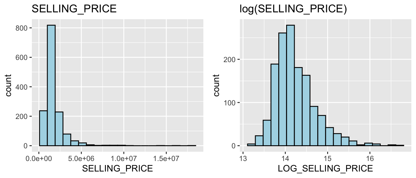
The raw price is strongly right-skewed; the log is close to symmetric. The handout derives the log and then models the raw price anyway. I follow it, because the point of the exercise is GWR rather than the best hedonic specification, but I return to the consequence in section 11.
6.2 The independent variables
vars <- c("AREA_SQM", "AGE", "PROX_CBD", "PROX_CHILDCARE",
"PROX_ELDERLYCARE", "PROX_URA_GROWTH_AREA",
"PROX_HAWKER_MARKET", "PROX_KINDERGARTEN", "PROX_MRT",
"PROX_PARK", "PROX_PRIMARY_SCH", "PROX_TOP_PRIMARY_SCH")
hists <- lapply(vars, function(v) {
ggplot(condo_resale.sf, aes(x = .data[[v]])) +
geom_histogram(bins = 20, color = "black", fill = "light blue") +
labs(x = v, y = NULL) +
theme(axis.title.x = element_text(size = 8))
})
ggarrange(plotlist = hists, ncol = 3, nrow = 4)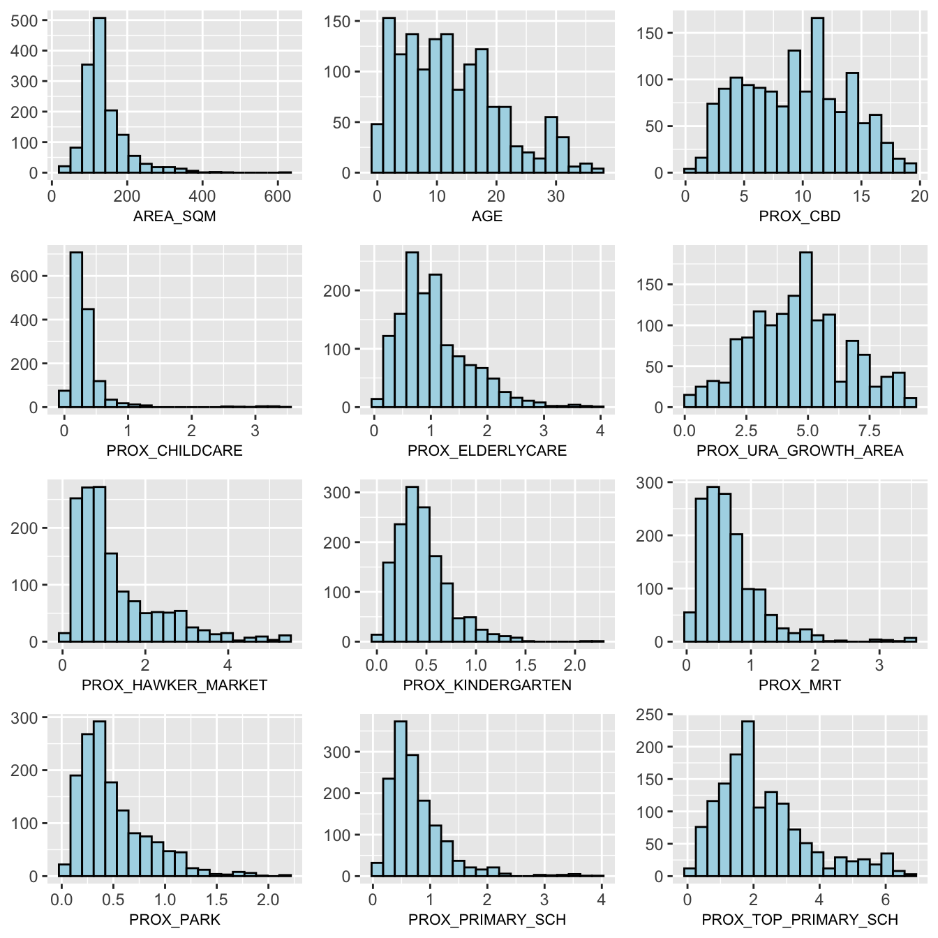
The handout builds these twelve histograms one assignment at a time. I build them in a loop over the variable names: same plots, and adding a variable is one word. Most proximity variables are right-skewed, as distances usually are: most condos are near a childcare centre or a bus stop and a few are far from everything.
6.3 Where the prices are
tmap_mode("plot")
tm_shape(mpsz_svy21) +
tm_polygons(fill = "grey95", col = "grey75", lwd = 0.3) +
tm_shape(condo_resale.sf) +
tm_dots(fill = "SELLING_PRICE",
fill_alpha = 0.7,
size = 0.25,
fill.scale = tm_scale_intervals(style = "quantile",
values = "brewer.yl_or_rd"),
fill.legend = tm_legend(title = "Selling price (S$)")) +
tm_layout(frame = FALSE)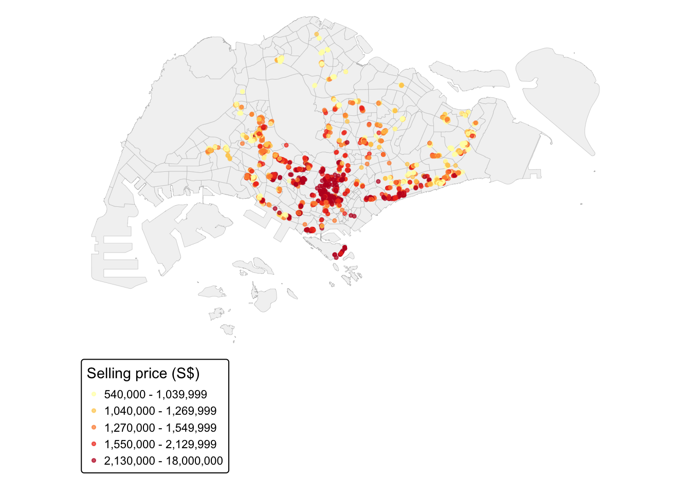
The handout draws this as an interactive map. I draw it static so the page stays light, and keep one interactive map for section 9.5 where zooming genuinely helps. The pattern is clear without zooming: the most expensive class is almost entirely in the Central Region. Joining the points to URA regions, 40% of Central Region transactions fall in the top price quintile, against 5% or less in every other region.
7. Hedonic Pricing with Ordinary Least Squares
7.1 Simple linear regression
condo.slr <- lm(SELLING_PRICE ~ AREA_SQM, data = condo_resale.sf)
summary(condo.slr)
Call:
lm(formula = SELLING_PRICE ~ AREA_SQM, data = condo_resale.sf)
Residuals:
Min 1Q Median 3Q Max
-3695815 -391764 -87517 258900 13503875
Coefficients:
Estimate Std. Error t value Pr(>|t|)
(Intercept) -258121.1 63517.2 -4.064 5.09e-05 ***
AREA_SQM 14719.0 428.1 34.381 < 2e-16 ***
---
Signif. codes: 0 '***' 0.001 '**' 0.01 '*' 0.05 '.' 0.1 ' ' 1
Residual standard error: 942700 on 1434 degrees of freedom
Multiple R-squared: 0.4518, Adjusted R-squared: 0.4515
F-statistic: 1182 on 1 and 1434 DF, p-value: < 2.2e-16ggplot(condo_resale.sf, aes(x = AREA_SQM, y = SELLING_PRICE)) +
geom_point(alpha = 0.4) +
geom_smooth(method = lm)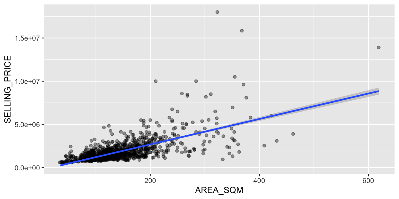
Floor area alone explains 45% of the variance in price. Each extra square metre adds about S$14,700. The scatterplot shows why the fit is not better: a band of very expensive units sits far above the line at every size, which is location speaking.
7.2 Checking for multicollinearity
corrplot(cor(condo_resale[, 5:23]),
diag = FALSE,
order = "AOE",
tl.pos = "td",
tl.cex = 0.5,
method = "number",
type = "upper")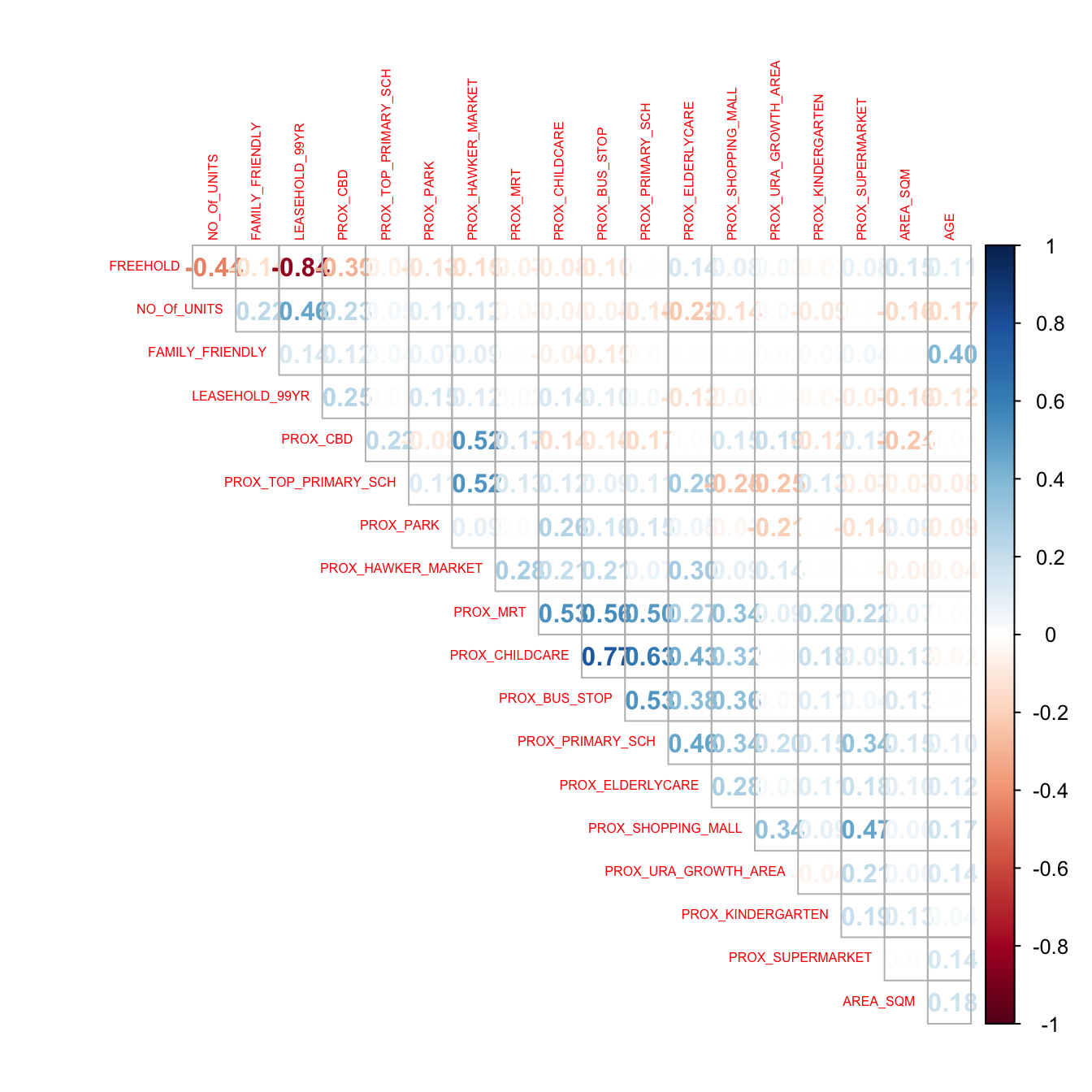
FREEHOLD and LEASEHOLD_99YR are strongly negatively correlated, which is close to true by definition: a unit that is not freehold is almost always on a 99-year lease. Keeping both would make their coefficients unstable, so LEASEHOLD_99YR is dropped.
7.3 The full multiple regression
condo.mlr <- lm(SELLING_PRICE ~ AREA_SQM + AGE +
PROX_CBD + PROX_CHILDCARE + PROX_ELDERLYCARE +
PROX_URA_GROWTH_AREA + PROX_HAWKER_MARKET +
PROX_KINDERGARTEN + PROX_MRT + PROX_PARK +
PROX_PRIMARY_SCH + PROX_TOP_PRIMARY_SCH +
PROX_SHOPPING_MALL + PROX_SUPERMARKET +
PROX_BUS_STOP + NO_Of_UNITS +
FAMILY_FRIENDLY + FREEHOLD,
data = condo_resale.sf)
summary(condo.mlr)
Call:
lm(formula = SELLING_PRICE ~ AREA_SQM + AGE + PROX_CBD + PROX_CHILDCARE +
PROX_ELDERLYCARE + PROX_URA_GROWTH_AREA + PROX_HAWKER_MARKET +
PROX_KINDERGARTEN + PROX_MRT + PROX_PARK + PROX_PRIMARY_SCH +
PROX_TOP_PRIMARY_SCH + PROX_SHOPPING_MALL + PROX_SUPERMARKET +
PROX_BUS_STOP + NO_Of_UNITS + FAMILY_FRIENDLY + FREEHOLD,
data = condo_resale.sf)
Residuals:
Min 1Q Median 3Q Max
-3475964 -293923 -23069 241043 12260381
Coefficients:
Estimate Std. Error t value Pr(>|t|)
(Intercept) 481728.40 121441.01 3.967 7.65e-05 ***
AREA_SQM 12708.32 369.59 34.385 < 2e-16 ***
AGE -24440.82 2763.16 -8.845 < 2e-16 ***
PROX_CBD -78669.78 6768.97 -11.622 < 2e-16 ***
PROX_CHILDCARE -351617.91 109467.25 -3.212 0.00135 **
PROX_ELDERLYCARE 171029.42 42110.51 4.061 5.14e-05 ***
PROX_URA_GROWTH_AREA 38474.53 12523.57 3.072 0.00217 **
PROX_HAWKER_MARKET 23746.10 29299.76 0.810 0.41782
PROX_KINDERGARTEN 147468.99 82668.87 1.784 0.07466 .
PROX_MRT -314599.68 57947.44 -5.429 6.66e-08 ***
PROX_PARK 563280.50 66551.68 8.464 < 2e-16 ***
PROX_PRIMARY_SCH 180186.08 65237.95 2.762 0.00582 **
PROX_TOP_PRIMARY_SCH 2280.04 20410.43 0.112 0.91107
PROX_SHOPPING_MALL -206604.06 42840.60 -4.823 1.57e-06 ***
PROX_SUPERMARKET -44991.80 77082.64 -0.584 0.55953
PROX_BUS_STOP 683121.35 138353.28 4.938 8.85e-07 ***
NO_Of_UNITS -231.18 89.03 -2.597 0.00951 **
FAMILY_FRIENDLY 140340.77 47020.55 2.985 0.00289 **
FREEHOLD 359913.01 49220.22 7.312 4.38e-13 ***
---
Signif. codes: 0 '***' 0.001 '**' 0.01 '*' 0.05 '.' 0.1 ' ' 1
Residual standard error: 755800 on 1417 degrees of freedom
Multiple R-squared: 0.6518, Adjusted R-squared: 0.6474
F-statistic: 147.4 on 18 and 1417 DF, p-value: < 2.2e-16Four variables are not significant at 5%: PROX_HAWKER_MARKET, PROX_KINDERGARTEN, PROX_TOP_PRIMARY_SCH and PROX_SUPERMARKET.
7.4 The revised model
condo.mlr1 <- lm(SELLING_PRICE ~ AREA_SQM + AGE +
PROX_CBD + PROX_CHILDCARE + PROX_MRT +
PROX_ELDERLYCARE + PROX_URA_GROWTH_AREA +
PROX_PARK + PROX_PRIMARY_SCH +
PROX_SHOPPING_MALL + PROX_BUS_STOP +
NO_Of_UNITS + FAMILY_FRIENDLY + FREEHOLD,
data = condo_resale.sf)
tbl_regression(condo.mlr1, intercept = TRUE) %>%
add_glance_source_note(
label = list(sigma ~ "\U03C3"),
include = c(r.squared, adj.r.squared,
AIC, statistic, p.value, sigma))| Characteristic | Beta | 95% CI | p-value |
|---|---|---|---|
| (Intercept) | 527,633 | 315,417, 739,849 | <0.001 |
| AREA_SQM | 12,778 | 12,057, 13,498 | <0.001 |
| AGE | -24,688 | -30,092, -19,284 | <0.001 |
| PROX_CBD | -77,131 | -88,436, -65,826 | <0.001 |
| PROX_CHILDCARE | -318,473 | -530,250, -106,696 | 0.003 |
| PROX_MRT | -294,745 | -406,394, -183,096 | <0.001 |
| PROX_ELDERLYCARE | 185,576 | 107,303, 263,849 | <0.001 |
| PROX_URA_GROWTH_AREA | 39,163 | 16,105, 62,222 | <0.001 |
| PROX_PARK | 570,505 | 442,004, 699,006 | <0.001 |
| PROX_PRIMARY_SCH | 159,856 | 41,698, 278,014 | 0.008 |
| PROX_SHOPPING_MALL | -220,947 | -292,668, -149,226 | <0.001 |
| PROX_BUS_STOP | 682,482 | 418,616, 946,348 | <0.001 |
| NO_Of_UNITS | -245 | -418, -73 | 0.005 |
| FAMILY_FRIENDLY | 146,308 | 54,321, 238,295 | 0.002 |
| FREEHOLD | 350,600 | 255,448, 445,752 | <0.001 |
| Abbreviation: CI = Confidence Interval | |||
| R² = 0.651; Adjusted R² = 0.647; AIC = 42,967; Statistic = 189; p-value = <0.001; σ = 755,957 | |||
Dropping the four costs almost nothing: adjusted R² moves from 0.6474 to 0.6472. Every remaining predictor is significant. Some signs are worth a second look rather than a nod. PROX_PRIMARY_SCH and PROX_PARK have positive coefficients, so price rises with distance from a primary school or a park, which runs against the family-buyer story. More likely those facilities are densest in the cheaper outer estates, while the most expensive condos sit in central districts with fewer of them. That is the first hint that one coefficient for the whole island is averaging over different markets.
7.5 Regression diagnostics
Multicollinearity
check_collinearity(condo.mlr1)# Check for Multicollinearity
Low Correlation
Term VIF VIF 95% CI adj. VIF Tolerance Tolerance 95% CI
AREA_SQM 1.15 [1.09, 1.23] 1.07 0.87 [0.81, 0.92]
AGE 1.41 [1.33, 1.52] 1.19 0.71 [0.66, 0.75]
PROX_CBD 1.57 [1.47, 1.69] 1.25 0.64 [0.59, 0.68]
PROX_CHILDCARE 3.26 [3.00, 3.56] 1.81 0.31 [0.28, 0.33]
PROX_MRT 1.91 [1.78, 2.07] 1.38 0.52 [0.48, 0.56]
PROX_ELDERLYCARE 1.52 [1.42, 1.63] 1.23 0.66 [0.61, 0.70]
PROX_URA_GROWTH_AREA 1.33 [1.26, 1.43] 1.15 0.75 [0.70, 0.80]
PROX_PARK 1.21 [1.15, 1.29] 1.10 0.83 [0.77, 0.87]
PROX_PRIMARY_SCH 2.21 [2.05, 2.40] 1.49 0.45 [0.42, 0.49]
PROX_SHOPPING_MALL 1.48 [1.39, 1.60] 1.22 0.67 [0.63, 0.72]
PROX_BUS_STOP 2.85 [2.62, 3.10] 1.69 0.35 [0.32, 0.38]
NO_Of_UNITS 1.45 [1.36, 1.56] 1.20 0.69 [0.64, 0.73]
FAMILY_FRIENDLY 1.38 [1.30, 1.48] 1.17 0.72 [0.67, 0.77]
FREEHOLD 1.44 [1.36, 1.55] 1.20 0.69 [0.65, 0.74]plot(check_collinearity(condo.mlr1))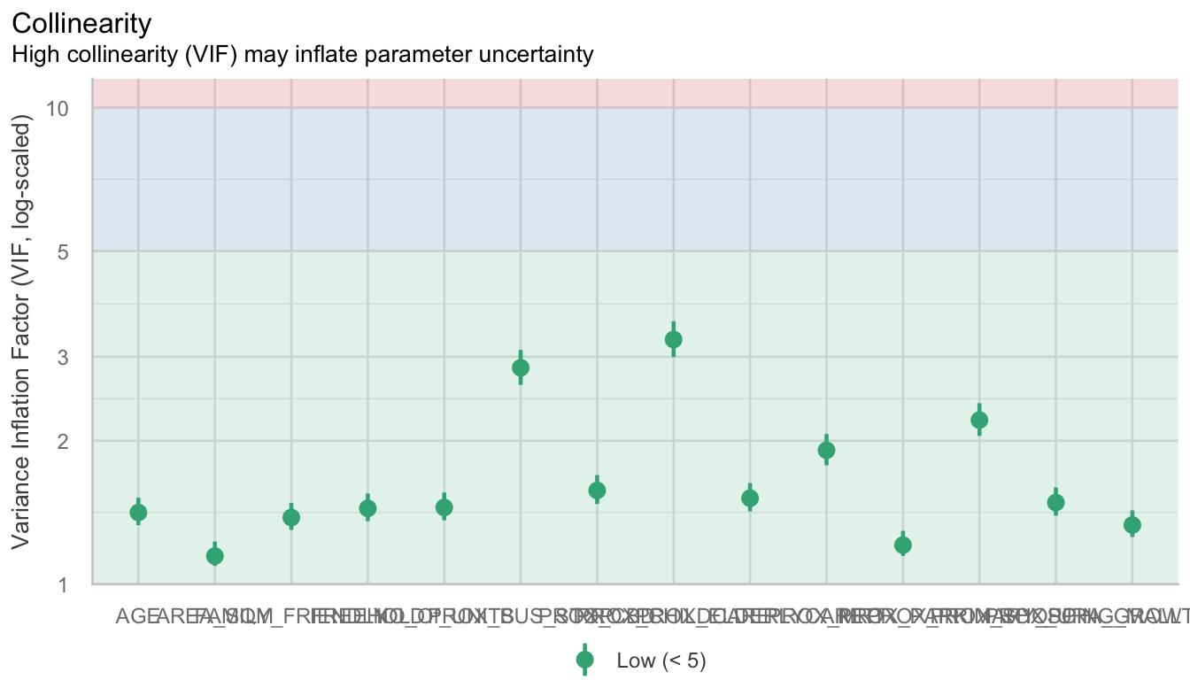
Every VIF is below 3.3, far from the conventional warning level of 5 or 10. Globally, collinearity is not a problem. Section 11.2 shows why that reassurance does not carry over to GWR.
Linearity
check_model(condo.mlr1, check = "linearity")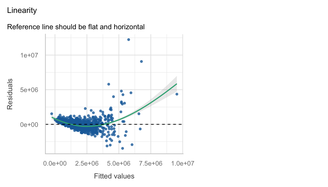
The residuals are centred on zero across most of the fitted range, with a fan at the expensive end. Linearity is acceptable; constant variance is not.
Normality of residuals
check_normality(condo.mlr1)Warning: Non-normality of residuals detected (p < .001).check_model(condo.mlr1, check = "normality")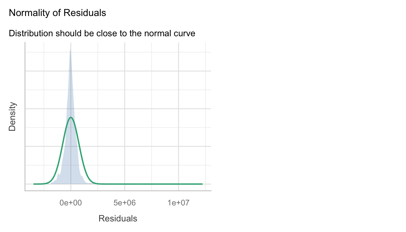
The Shapiro-Wilk test rejects normality decisively. The handout reads the density plot as roughly normal, and it is in the middle. The tails are not: the Q-Q plot bends away at both ends, the signature of the long upper tail from section 6.1.
7.6 Spatial autocorrelation in the residuals
This is the test that motivates GWR. If the model has captured everything that matters, its errors should be spatially random. If location still matters, residuals will cluster.
condo_resale.sf <- cbind(condo_resale.sf,
condo.mlr1$residuals) %>%
rename(MLR_RES = condo.mlr1.residuals)tm_shape(mpsz_svy21) +
tm_polygons(fill = "grey95", col = "grey75", lwd = 0.3) +
tm_shape(condo_resale.sf) +
tm_dots(fill = "MLR_RES",
size = 0.25,
fill.scale = tm_scale_intervals(
n = 10, style = "quantile",
values = rev(brewer.pal(11, "RdBu"))),
fill.legend = tm_legend(title = "OLS residual")) +
tm_title("OLS residuals (quantile classes)") +
tm_layout(frame = FALSE, legend.outside = TRUE)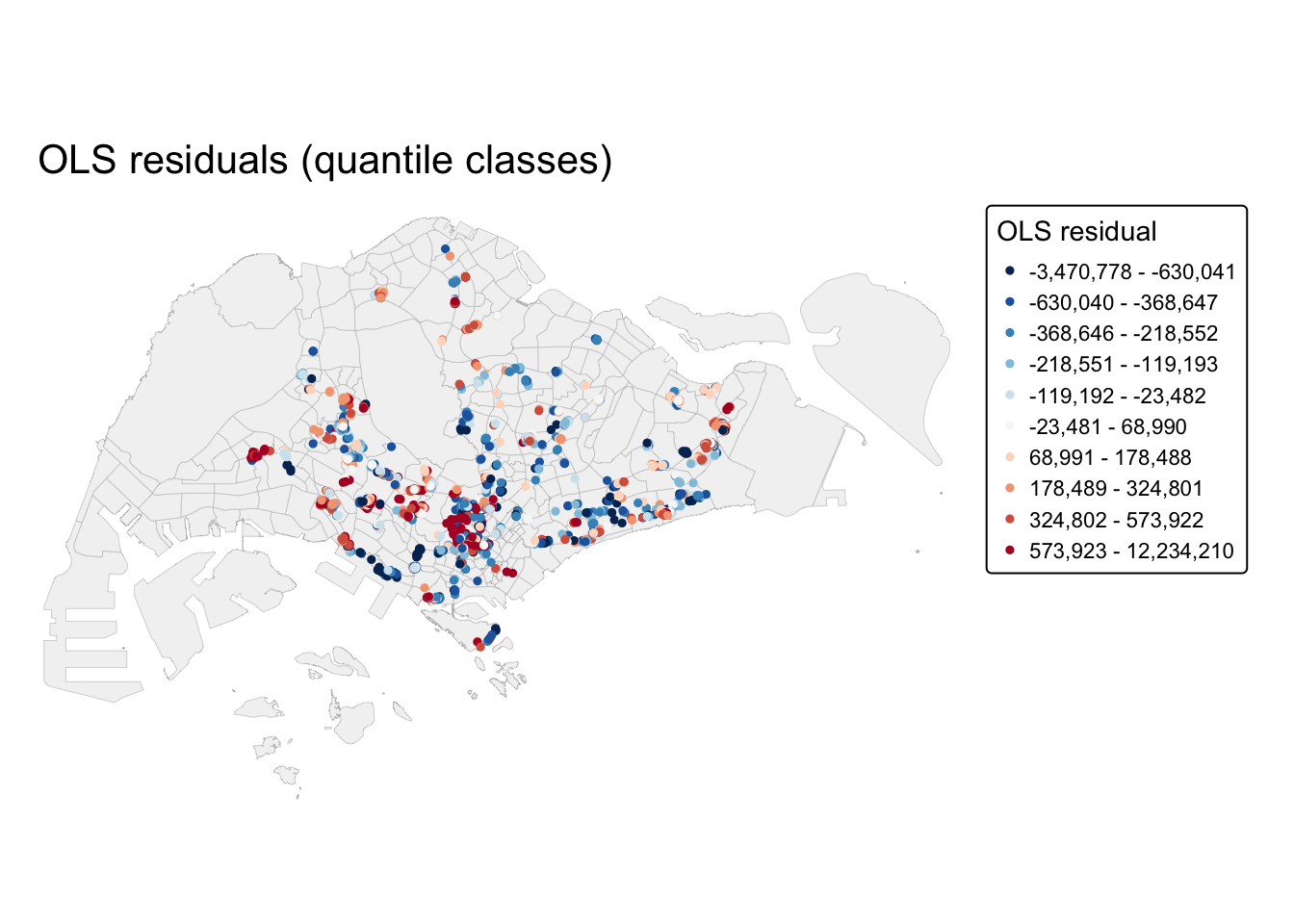
Red points are under-predicted (they sold for more than the model says), blue over-predicted. They are not scattered at random. Counting by URA region, 80% of North Region residuals are positive and 68% of North-East Region residuals are negative: the global model systematically under-prices one area and over-prices another.
condo_resale.sf <- condo_resale.sf %>%
mutate(nb = st_dist_band(st_geometry(geometry), upper = 1500),
wt = st_weights(nb, style = "W"),
.before = 1)
set.seed(1234)
global_moran_perm(condo_resale.sf$MLR_RES,
nb = condo_resale.sf$nb,
wt = condo_resale.sf$wt,
alternative = "two.sided",
nsim = 499)
Monte-Carlo simulation of Moran I
data: x
weights: listw
number of simulations + 1: 500
statistic = 0.14389, observed rank = 500, p-value < 2.2e-16
alternative hypothesis: two.sidedMoran’s I is 0.144 with every one of 499 permutations below it. The residuals are clustered. The global model has left location-specific structure in its errors, which is exactly the condition GWR is designed for.
8. A Short Note on GWmodel
GWmodel provides a family of geographically weighted methods: summary statistics, principal components, discriminant analysis, and several forms of GWR (basic, robust, generalised, mixed, and multiscale). This exercise uses the basic form, gwr.basic(), with its bandwidth selector bw.gwr().
9. Geographically Weighted Regression
The bandwidth decides how many observations each local regression sees. Too wide and GWR collapses back to the global model; too narrow and each local fit is estimated from a handful of points and chases noise. bw.gwr() chooses it by cross-validation: leave each observation out, predict it from its neighbours, and pick the bandwidth that minimises the squared prediction error.
There are two ways to define “neighbourhood”. A fixed bandwidth uses the same distance everywhere. An adaptive bandwidth uses the same number of neighbours everywhere, so the radius stretches where condos are sparse and shrinks where they are dense.
9.1 Fixed bandwidth
bw.fixed <- bw.gwr(
formula = SELLING_PRICE ~ AREA_SQM + AGE +
PROX_CBD + PROX_CHILDCARE + PROX_ELDERLYCARE +
PROX_URA_GROWTH_AREA + PROX_MRT + PROX_PARK +
PROX_PRIMARY_SCH + PROX_SHOPPING_MALL +
PROX_BUS_STOP + NO_Of_UNITS + FAMILY_FRIENDLY +
FREEHOLD,
data = condo_resale.sf,
approach = "CV",
kernel = "gaussian",
adaptive = FALSE,
longlat = FALSE)bw.fixed[1] 971.3393I hide the cross-validation trace, which prints dozens of lines of CV scores. The chosen bandwidth is about 971 m. My run lands on 971.34 m, which matches the handout’s text; the handout’s printed output shows 971.39 m. The difference is the stopping tolerance of the golden-section search, half a metre either way, and has no effect on anything below.
gwr.fixed <- gwr.basic(
formula = SELLING_PRICE ~ AREA_SQM + AGE +
PROX_CBD + PROX_CHILDCARE + PROX_ELDERLYCARE +
PROX_URA_GROWTH_AREA + PROX_MRT + PROX_PARK +
PROX_PRIMARY_SCH + PROX_SHOPPING_MALL +
PROX_BUS_STOP + NO_Of_UNITS + FAMILY_FRIENDLY +
FREEHOLD,
data = condo_resale.sf,
bw = bw.fixed,
kernel = "gaussian",
longlat = FALSE)
gwr.fixed ***********************************************************************
* Package GWmodel *
***********************************************************************
Program starts at: 2026-10-30 17:35:09.668069
Call:
gwr.basic(formula = SELLING_PRICE ~ AREA_SQM + AGE + PROX_CBD +
PROX_CHILDCARE + PROX_ELDERLYCARE + PROX_URA_GROWTH_AREA +
PROX_MRT + PROX_PARK + PROX_PRIMARY_SCH + PROX_SHOPPING_MALL +
PROX_BUS_STOP + NO_Of_UNITS + FAMILY_FRIENDLY + FREEHOLD,
data = condo_resale.sf, bw = bw.fixed, kernel = "gaussian",
longlat = FALSE)
Dependent (y) variable: SELLING_PRICE
Independent variables: AREA_SQM AGE PROX_CBD PROX_CHILDCARE PROX_ELDERLYCARE PROX_URA_GROWTH_AREA PROX_MRT PROX_PARK PROX_PRIMARY_SCH PROX_SHOPPING_MALL PROX_BUS_STOP NO_Of_UNITS FAMILY_FRIENDLY FREEHOLD
Number of data points: 1436
***********************************************************************
* Results of Global Regression *
***********************************************************************
Call:
lm(formula = formula, data = data)
Residuals:
Min 1Q Median 3Q Max
-3470778 -298119 -23481 248917 12234210
Coefficients:
Estimate Std. Error t value Pr(>|t|)
(Intercept) 527633.22 108183.22 4.877 1.20e-06 ***
AREA_SQM 12777.52 367.48 34.771 < 2e-16 ***
AGE -24687.74 2754.84 -8.962 < 2e-16 ***
PROX_CBD -77131.32 5763.12 -13.384 < 2e-16 ***
PROX_CHILDCARE -318472.75 107959.51 -2.950 0.003231 **
PROX_ELDERLYCARE 185575.62 39901.86 4.651 3.61e-06 ***
PROX_URA_GROWTH_AREA 39163.25 11754.83 3.332 0.000885 ***
PROX_MRT -294745.11 56916.37 -5.179 2.56e-07 ***
PROX_PARK 570504.81 65507.03 8.709 < 2e-16 ***
PROX_PRIMARY_SCH 159856.14 60234.60 2.654 0.008046 **
PROX_SHOPPING_MALL -220947.25 36561.83 -6.043 1.93e-09 ***
PROX_BUS_STOP 682482.22 134513.24 5.074 4.42e-07 ***
NO_Of_UNITS -245.48 87.95 -2.791 0.005321 **
FAMILY_FRIENDLY 146307.58 46893.02 3.120 0.001845 **
FREEHOLD 350599.81 48506.48 7.228 7.98e-13 ***
---Significance stars
Signif. codes: 0 '***' 0.001 '**' 0.01 '*' 0.05 '.' 0.1 ' ' 1
Residual standard error: 756000 on 1421 degrees of freedom
Multiple R-squared: 0.6507
Adjusted R-squared: 0.6472
F-statistic: 189.1 on 14 and 1421 DF, p-value: < 2.2e-16
***Extra Diagnostic information
Residual sum of squares: 8.120609e+14
Sigma(hat): 752522.9
AIC: 42966.76
AICc: 42967.14
BIC: 41731.39
***********************************************************************
* Results of Geographically Weighted Regression *
***********************************************************************
*********************Model calibration information*********************
Kernel function: gaussian
Fixed bandwidth: 971.3393
Regression points: the same locations as observations are used.
Distance metric: Euclidean distance metric is used.
****************Summary of GWR coefficient estimates:******************
Min. 1st Qu. Median 3rd Qu.
Intercept -3.5988e+07 -5.1998e+05 7.6779e+05 1.7412e+06
AREA_SQM 1.0003e+03 5.2758e+03 7.4740e+03 1.2301e+04
AGE -1.3475e+05 -2.0813e+04 -8.6260e+03 -3.7784e+03
PROX_CBD -7.7047e+07 -2.3608e+05 -8.3599e+04 3.4647e+04
PROX_CHILDCARE -6.0097e+06 -3.3667e+05 -9.7426e+04 2.9007e+05
PROX_ELDERLYCARE -3.5001e+06 -1.5970e+05 3.1970e+04 1.9578e+05
PROX_URA_GROWTH_AREA -3.0170e+06 -8.2013e+04 7.0749e+04 2.2612e+05
PROX_MRT -3.5282e+06 -6.5836e+05 -1.8833e+05 3.6923e+04
PROX_PARK -1.2062e+06 -2.1732e+05 3.5383e+04 4.1335e+05
PROX_PRIMARY_SCH -2.2695e+07 -1.7066e+05 4.8472e+04 5.1555e+05
PROX_SHOPPING_MALL -7.2585e+06 -1.6684e+05 -1.0516e+04 1.5923e+05
PROX_BUS_STOP -1.4676e+06 -4.5208e+04 3.7601e+05 1.1664e+06
NO_Of_UNITS -1.3170e+03 -2.4822e+02 -3.0846e+01 2.5496e+02
FAMILY_FRIENDLY -2.2749e+06 -1.1140e+05 7.6214e+03 1.6107e+05
FREEHOLD -9.2068e+06 3.8074e+04 1.5169e+05 3.7528e+05
Max.
Intercept 112795537
AREA_SQM 21575
AGE 434205
PROX_CBD 2704613
PROX_CHILDCARE 1654084
PROX_ELDERLYCARE 38867918
PROX_URA_GROWTH_AREA 78515898
PROX_MRT 3124337
PROX_PARK 18122457
PROX_PRIMARY_SCH 4637533
PROX_SHOPPING_MALL 1529955
PROX_BUS_STOP 11342241
NO_Of_UNITS 12907
FAMILY_FRIENDLY 1720746
FREEHOLD 6073649
************************Diagnostic information*************************
Number of data points: 1436
Effective number of parameters (2trace(S) - trace(S'S)): 438.381
Effective degrees of freedom (n-2trace(S) + trace(S'S)): 997.619
AICc (GWR book, Fotheringham, et al. 2002, p. 61, eq 2.33): 42263.61
AIC (GWR book, Fotheringham, et al. 2002,GWR p. 96, eq. 4.22): 41632.36
BIC (GWR book, Fotheringham, et al. 2002,GWR p. 61, eq. 2.34): 42515.71
Residual sum of squares: 2.534067e+14
R-square value: 0.8909913
Adjusted R-square value: 0.8430418
***********************************************************************
Program stops at: 2026-10-30 17:35:11.313594 9.2 Adaptive bandwidth
bw.adaptive <- bw.gwr(
formula = SELLING_PRICE ~ AREA_SQM + AGE +
PROX_CBD + PROX_CHILDCARE + PROX_ELDERLYCARE +
PROX_URA_GROWTH_AREA + PROX_MRT + PROX_PARK +
PROX_PRIMARY_SCH + PROX_SHOPPING_MALL +
PROX_BUS_STOP + NO_Of_UNITS +
FAMILY_FRIENDLY + FREEHOLD,
data = condo_resale.sf,
approach = "CV",
kernel = "gaussian",
adaptive = TRUE,
longlat = FALSE)bw.adaptive[1] 30gwr.adaptive <- gwr.basic(
formula = SELLING_PRICE ~ AREA_SQM + AGE +
PROX_CBD + PROX_CHILDCARE + PROX_ELDERLYCARE +
PROX_URA_GROWTH_AREA + PROX_MRT + PROX_PARK +
PROX_PRIMARY_SCH + PROX_SHOPPING_MALL + PROX_BUS_STOP +
NO_Of_UNITS + FAMILY_FRIENDLY + FREEHOLD,
data = condo_resale.sf,
bw = bw.adaptive,
kernel = "gaussian",
adaptive = TRUE,
longlat = FALSE)
gwr.adaptive ***********************************************************************
* Package GWmodel *
***********************************************************************
Program starts at: 2026-10-30 17:35:23.249367
Call:
gwr.basic(formula = SELLING_PRICE ~ AREA_SQM + AGE + PROX_CBD +
PROX_CHILDCARE + PROX_ELDERLYCARE + PROX_URA_GROWTH_AREA +
PROX_MRT + PROX_PARK + PROX_PRIMARY_SCH + PROX_SHOPPING_MALL +
PROX_BUS_STOP + NO_Of_UNITS + FAMILY_FRIENDLY + FREEHOLD,
data = condo_resale.sf, bw = bw.adaptive, kernel = "gaussian",
adaptive = TRUE, longlat = FALSE)
Dependent (y) variable: SELLING_PRICE
Independent variables: AREA_SQM AGE PROX_CBD PROX_CHILDCARE PROX_ELDERLYCARE PROX_URA_GROWTH_AREA PROX_MRT PROX_PARK PROX_PRIMARY_SCH PROX_SHOPPING_MALL PROX_BUS_STOP NO_Of_UNITS FAMILY_FRIENDLY FREEHOLD
Number of data points: 1436
***********************************************************************
* Results of Global Regression *
***********************************************************************
Call:
lm(formula = formula, data = data)
Residuals:
Min 1Q Median 3Q Max
-3470778 -298119 -23481 248917 12234210
Coefficients:
Estimate Std. Error t value Pr(>|t|)
(Intercept) 527633.22 108183.22 4.877 1.20e-06 ***
AREA_SQM 12777.52 367.48 34.771 < 2e-16 ***
AGE -24687.74 2754.84 -8.962 < 2e-16 ***
PROX_CBD -77131.32 5763.12 -13.384 < 2e-16 ***
PROX_CHILDCARE -318472.75 107959.51 -2.950 0.003231 **
PROX_ELDERLYCARE 185575.62 39901.86 4.651 3.61e-06 ***
PROX_URA_GROWTH_AREA 39163.25 11754.83 3.332 0.000885 ***
PROX_MRT -294745.11 56916.37 -5.179 2.56e-07 ***
PROX_PARK 570504.81 65507.03 8.709 < 2e-16 ***
PROX_PRIMARY_SCH 159856.14 60234.60 2.654 0.008046 **
PROX_SHOPPING_MALL -220947.25 36561.83 -6.043 1.93e-09 ***
PROX_BUS_STOP 682482.22 134513.24 5.074 4.42e-07 ***
NO_Of_UNITS -245.48 87.95 -2.791 0.005321 **
FAMILY_FRIENDLY 146307.58 46893.02 3.120 0.001845 **
FREEHOLD 350599.81 48506.48 7.228 7.98e-13 ***
---Significance stars
Signif. codes: 0 '***' 0.001 '**' 0.01 '*' 0.05 '.' 0.1 ' ' 1
Residual standard error: 756000 on 1421 degrees of freedom
Multiple R-squared: 0.6507
Adjusted R-squared: 0.6472
F-statistic: 189.1 on 14 and 1421 DF, p-value: < 2.2e-16
***Extra Diagnostic information
Residual sum of squares: 8.120609e+14
Sigma(hat): 752522.9
AIC: 42966.76
AICc: 42967.14
BIC: 41731.39
***********************************************************************
* Results of Geographically Weighted Regression *
***********************************************************************
*********************Model calibration information*********************
Kernel function: gaussian
Adaptive bandwidth: 30 (number of nearest neighbours)
Regression points: the same locations as observations are used.
Distance metric: Euclidean distance metric is used.
****************Summary of GWR coefficient estimates:******************
Min. 1st Qu. Median 3rd Qu.
Intercept -1.3487e+08 -2.4669e+05 7.7928e+05 1.6194e+06
AREA_SQM 3.3188e+03 5.6285e+03 7.7825e+03 1.2738e+04
AGE -9.6746e+04 -2.9288e+04 -1.4043e+04 -5.6119e+03
PROX_CBD -2.5330e+06 -1.6256e+05 -7.7242e+04 2.6624e+03
PROX_CHILDCARE -1.2790e+06 -2.0175e+05 8.7158e+03 3.7778e+05
PROX_ELDERLYCARE -1.6212e+06 -9.2050e+04 6.1029e+04 2.8184e+05
PROX_URA_GROWTH_AREA -7.2686e+06 -3.0350e+04 4.5869e+04 2.4613e+05
PROX_MRT -4.3781e+07 -6.7282e+05 -2.2115e+05 -7.4593e+04
PROX_PARK -2.9020e+06 -1.6782e+05 1.1601e+05 4.6572e+05
PROX_PRIMARY_SCH -8.6418e+05 -1.6627e+05 -7.7853e+03 4.3222e+05
PROX_SHOPPING_MALL -1.8272e+06 -1.3175e+05 -1.4049e+04 1.3799e+05
PROX_BUS_STOP -2.0579e+06 -7.1461e+04 4.1104e+05 1.2071e+06
NO_Of_UNITS -2.1993e+03 -2.3685e+02 -3.4699e+01 1.1657e+02
FAMILY_FRIENDLY -5.9879e+05 -5.0927e+04 2.6173e+04 2.2481e+05
FREEHOLD -1.6340e+05 4.0765e+04 1.9023e+05 3.7960e+05
Max.
Intercept 18758355
AREA_SQM 23064
AGE 13303
PROX_CBD 11346650
PROX_CHILDCARE 2892127
PROX_ELDERLYCARE 2465671
PROX_URA_GROWTH_AREA 7384059
PROX_MRT 1186242
PROX_PARK 2588497
PROX_PRIMARY_SCH 3381462
PROX_SHOPPING_MALL 38038564
PROX_BUS_STOP 12081592
NO_Of_UNITS 1010
FAMILY_FRIENDLY 2072414
FREEHOLD 1813995
************************Diagnostic information*************************
Number of data points: 1436
Effective number of parameters (2trace(S) - trace(S'S)): 350.3088
Effective degrees of freedom (n-2trace(S) + trace(S'S)): 1085.691
AICc (GWR book, Fotheringham, et al. 2002, p. 61, eq 2.33): 41982.22
AIC (GWR book, Fotheringham, et al. 2002,GWR p. 96, eq. 4.22): 41546.74
BIC (GWR book, Fotheringham, et al. 2002,GWR p. 61, eq. 2.34): 41914.08
Residual sum of squares: 2.528227e+14
R-square value: 0.8912425
Adjusted R-square value: 0.8561185
***********************************************************************
Program stops at: 2026-10-30 17:35:25.349194 9.3 Comparing the three models
tibble(
model = c("OLS (global)", "GWR, fixed bandwidth", "GWR, adaptive bandwidth"),
bandwidth = c("-", paste(round(bw.fixed), "m"), paste(bw.adaptive, "neighbours")),
# AICc for OLS: AIC plus the small-sample correction, with k = 16
# (15 coefficients and the residual variance)
AICc = c(AIC(condo.mlr1) + 2 * 16 * 17 / (nrow(condo_resale.sf) - 16 - 1),
gwr.fixed$GW.diagnostic$AICc, gwr.adaptive$GW.diagnostic$AICc),
adj_R2 = c(summary(condo.mlr1)$adj.r.squared,
gwr.fixed$GW.diagnostic$gwR2.adj, gwr.adaptive$GW.diagnostic$gwR2.adj),
effective_parameters = c(15, gwr.fixed$GW.diagnostic$enp, gwr.adaptive$GW.diagnostic$enp)
) %>% mutate(across(c(AICc, adj_R2, effective_parameters), \(x) round(x, 3)))# A tibble: 3 x 5
model bandwidth AICc adj_R2 effective_parameters
<chr> <chr> <dbl> <dbl> <dbl>
1 OLS (global) - 42967. 0.647 15
2 GWR, fixed bandwidth 971 m 42264. 0.843 438.
3 GWR, adaptive bandwidth 30 neighbours 41982. 0.856 350.Both GWR models improve on the global model by a wide margin: AICc falls by about 700 (fixed) and 985 (adaptive), and adjusted R² rises from 0.65 to 0.84 and 0.86. AICc penalises the extra effective parameters, so this is not just a more flexible model fitting better; it is a better model after paying for the flexibility.
The adaptive model wins on every measure and uses fewer effective parameters (350 against 438). That makes sense for Singapore condos, which are dense in the centre and sparse at the edges: a fixed 971 m window holds dozens of transactions in the core and only a few on the periphery, while 30 neighbours gives every local fit the same amount of evidence.
9.4 Converting the output to sf
condo_resale.sf.adaptive <- st_as_sf(gwr.adaptive$SDF) %>%
st_transform(crs = 3414)
summary(gwr.adaptive$SDF$yhat) Min. 1st Qu. Median Mean 3rd Qu. Max.
171347 1102001 1385528 1751842 1982307 13887901 The SDF holds, for every transaction, its local coefficients, their standard errors and t-values, the fitted value, the residual and a local R².
9.5 Local R²
tmap_mode("view")
tm_shape(mpsz_svy21) +
tm_polygons(fill_alpha = 0.1) +
tm_shape(condo_resale.sf.adaptive) +
tm_dots(fill = "Local_R2",
size = 0.15,
fill.scale = tm_scale_intervals(style = "quantile",
values = "brewer.blues")) +
tm_view(set_zoom_limits = c(11, 14))